Basic Differentiation

Before we study the differentiation of single-variable functions, we briefly review several foundational mathematical concepts.

Functions¶

A function $f$ from a set $X$ to a set $Y$ , written $f: X \to Y$ , is a rule that assigns exactly one element of $Y$ to each element of $X$ .

$X$ is called the domain
The range is the set of values in $Y$ that are actually attained

Using $x \in X$ and $y \in Y$ , a function is written as $y = f(x)$ , where $x$ is the independent variable and $y$ the dependent variable.

Graphs¶

If $X$ and $Y$ are sets of real numbers, the graph of a function $f$ is the set of points $(x, y)$ such that $y = f(x)$ .

Economic convention.
Economists often draw demand curves with quantity on the horizontal axis and price on the vertical axis, even when the function is written as $q = f(p)$ .

Slope¶

The slope of a line through points $(x, y)$ and $(x', y')$ is

m = \frac{y' - y}{x' - x}.

Differentiation is the method of finding the slope of a function and is denoted by $f'(x)$ .

Limits¶

We say that a function $f$ has limit $L$ as $x \to a$ if, for any $\varepsilon > 0$ , there exists a $\delta > 0$ such that^[1]

|f(x) - L| < \varepsilon \quad \text{whenever} \quad 0 < |x - a| < \delta.

When this condition holds, we write

\lim_{x \to a} f(x) = L.

Continuity¶

A function $f$ is continuous at $a$ if:^[2]

$f(a)$ is defined
$\lim_{x \to a} f(x)$ exists
$\lim_{x \to a} f(x) = f(a)$

Derivative at a Point¶

Let $y = f(x)$ . When $x$ changes by $\Delta x$ , the change in $y$ is

\frac{\Delta y}{\Delta x} = \frac{f(x+\Delta x) - f(x)}{\Delta x}.

Derivative as a Function¶

The derivative of $f$ at $x$ is defined as

f'(x) = \lim_{\Delta x \to 0} \frac{f(x+\Delta x) - f(x)}{\Delta x}.

If the derivative exists for every $x$ in the domain of $f$ , then the derivative itself defines a new function, denoted $f'(x)$ .

Geometrically, $f'(x)$ is the slope of the tangent line to the graph of $f$ at $(x, f(x))$ .

Common notations include:

$f'(x)$
$\dfrac{dy}{dx}$
$Df(x)$

Note that what we usually think of as a variable $x$ is held constant while $\Delta x$ varies and converges to zero. It is useful to keep in mind that the derivative of a function $f$ at $x$ is the slope of a line tangent to the graph of the function $f$ at the point $(x, f(x))$ . It is crucial to understand the implications of the existence of the derivative at a point $x$ . The function must be smooth—meaning it is both continuous and differentiable—at the point $x$ . The tangent line provides a high-quality linear approximation to the graph of the function near $x$ . In general, if we know that the function $f$ is differentiable at $a$ , then the tangent line approximation to $f$ at $a$ is:

y = f(a) + f'(a)(x - a)

where $a, f(a), \text{ and } f'(a)$ are constants, $x$ is the independent variable, and $y$ is the dependent variable. We will see this point again with Taylor series expansions. Many important concepts in economics—such as marginal cost or marginal utility—are based on this derivative function.

Second Derivative¶

The second derivative is the derivative of the derivative and is written as

f''(x) = \frac{d^2 f(x)}{dx^2}.

Economic interpretation.
If $\ln p(t)$ describes log prices over time, then:
the first derivative is inflation
the second derivative is the change in inflation

Basic Rules of Differentiation¶

Let $y = f(x)$ .

Constant-function Rule¶

The derivative of a contsant function $y=f(x)=k$ is zero, for all values of x-it has zero slope!

\frac{d}{dx}(k) = 0.

Power-function Rule¶

The derivative of a power function $f(x) = x^n$ is:

\frac{d}{dx}(x^n) = n x^{n-1}.

Generalized Power-function Rule¶

When a multiplicaytive constant $k$ appears in the power fuction, so that $f(x) = kx^n$ , then:

\frac{d}{dx}(k x^n) = k n x^{n-1}.

Logarithmic Rule¶

The derivatice of the log-function $f(x) = lnx$ is:

\frac{d}{dx}(\ln x) = \frac{1}{x}.

Exponential Rule¶

For some exponential function $f(x) = a^x$ , where $a$ is some constant, then:

\frac{d}{dx}(a^x) = a^x \ln a.

Note that a particular case of the above is

\frac{d}{d x} e^x = e^x

While

\frac{d}{d x} \ln x = \frac{1}{x}

Now, let’s consider some further useful rules of differentiation involving two or more functions of the same variable. Specifically, suppose $f(x)$ and $g(x)$ are two different functions of $x$ and that $f'(x)$ and $g'(x)$ exist. That is, let $f(x)$ and $g(x)$ be differentiable, then:

Sum-difference Rules¶

The derivative of a sum (difference) of two functions is the sum (difference) of the derivatives of the two functions.

\frac{d}{dx}[f(x) \pm g(x)] = f'(x) \pm g'(x).

Product Rule¶

The derivative of the product of two (differentiable) functions is equal to the first function times the derivative of the second function plus the second function times the derivative of the first function.

\frac{d}{dx}[f(x)g(x)] = f'(x)g(x) + f(x)g'(x).

Quotient Rule¶

The derivative of the quotient of two (differentiable) functions, $f(x)/g(x)$ , is

\frac{d}{dx} \left[ \frac{f(x)}{g(x)} \right] = \frac{g(x)f'(x) - f(x)g'(x)}{[g(x)]^2}

provided that $g(x) \neq 0$ . Note that $[g(x)]^2 = g^2(x)$ .

Chain Rule¶

If $z = f(y)$ and $y = g(x)$ , then

\frac{dz}{dx} = \frac{dz}{dy}\frac{dy}{dx}.

The chain rule provides a convenient way to study how one variable (say, $x$ ) affects another variable ( $z$ ) through its influence on some intermediate variable ( $y$ ).

Sometimes, we can write for a composite function $y = f(g(x))$ :

\frac{dy}{dx} = f'(g(x)) \cdot g'(x)

Chain Rule for Exponential and Logarithmic Functions¶

The general exponential function rule¶

\frac{d}{d x} e^{g(x)} = e^{g(x)} g'(x)

For example:

\frac{d}{d x} e^{ax} = \frac{d}{d (ax)} e^{ax} \frac{d}{d x} (ax) = e^{ax} a = ae^{ax}

If we are using a base other than $e$ :

\frac {d}{d x}(a^{g(x)}) = a^{g(x)} g'(x) \ln a, \text{ where } a > 0, a \neq 0

The general natural logarithmic function rule¶

\frac{d}{d x} \ln(g(x)) = \frac{g'(x)}{g(x)}

Interestingly:

\frac{d}{d x} \ln(ax) = \frac{d}{d(ax)} \ln(ax) \frac{d}{d x}(ax) = \frac{1}{ax} a = 1/x

while

\frac{d}{d x} \ln(x^2) = \frac{d}{d(x^2)} \ln(x^2) \frac{d}{d x}(x^2) = \frac{1}{x^2} 2x = 2/x

Note also when considered base other than $e$ . Because

\log_b(x) = \frac{\ln(x)}{\ln(b)}

we have

\frac{d}{d x} \log_b(x) = \frac{1}{x} \frac{1}{\ln(b)}

Or more generally:

\begin{aligned} \frac{d}{d x} \log_b g(x) &= \frac{g'(x)}{g(x)} \frac{1}{\ln b}, \text{ where } b > 0, b \neq 1 \\ &= \frac{g'(x)}{g(x)} \log_b e \end{aligned}

Note that $\log_b e = \displaystyle \frac{1}{\ln b}$ .

Exponential Functions

Use the rules of differentiating exponential functions to find the derivative with respect to $x$ of each of the following functions.

$y = x^2 e^{5x}$
$y = \dfrac{e^{5x}-1}{e^{5x}+1}$
$y = a^{2x}$
$y = a^{5x^2}$
$y = 4^{2x+7}$
$y = x^3 2^x$

Answers

$1.\; y' = x e^{5x}(5x+2) \quad 2.\; y' = \frac{10e^{5x}}{(e^{5x}+1)^2} \quad 3.\; y' = 2a^{2x}\ln a \quad 4.\; y' = 10x\,a^{5x^2}\ln a \quad 5.\; y' = 2\ln(4)\,4^{2x+7} \quad 6.\; y' = x^2 2^x(x\ln 2 + 3)$

Logarithmic Functions

Use the rules of differentiating logarithms to find the derivative of each function.

$f(x)=x^{-4}+\ln(ax)$
$f(x)=4x^3\ln x^2$
$f(x)=\ln x-\ln(1+x)$
$f(x)=\ln\!\left(\dfrac{2x^2}{5x}\right)$
$f(x)=\log_2(6x)$
$f(x)=\log_4(9x^3)$

Answers

$1.\; f'(x)=-4x^{-5}+x^{-1} \quad 2.\; f'(x)=8x^2+24x^2\ln x \quad 3.\; f'(x)=\frac{1}{x(1+x)} \quad 4.\; f'(x)=\frac{1}{x} \quad 5.\; f'(x)=\frac{1}{x\ln 2} \quad 6.\; f'(x)=\frac{3}{x\ln 4}$

Chain Rule

Use the chain rule to find the derivative, $f'(x)$ , of the following:

$f(x) = (x + 1)^3 + (x^2 - 2x)^2 - 5$
$f(x) = (2x + 4)^{99}$
$f(x) = (5x^2 + 10x + 3)^{20}$
$f(x) = (e^x)^{ab}$
$f(x) = (e^{x^a})^{b}$
$f(x) = (e^{a + bx + cx^2})^{10}$

Answers

$1.\; f'(x)=4x^3-9x^2+14x+3 \quad 2.\; f'(x)=198(2x+4)^{98} \quad 3.\; f'(x)=(200x+200)(5x^2+10x+3)^{19} \\[6pt] 4.\; f'(x)=ab\,e^{abx} \quad 5.\; f'(x)=ab\,x^{a-1}e^{bx^a} \quad 6.\; f'(x)=10(b+2cx)(e^{a+bx+cx^2})^{10}$

Derivatives of Exponential and Logarithmic Functions

1. Exponential Rule with Base $a$

Problem: Find the derivative of $f(x) = 5^{x^3 + 2x}$ .

Solution: Using the rule $\frac{d}{d x}(a^{g(x)}) = a^{g(x)} g'(x) \ln a$ :

Let $a = 5$
Let $g(x) = x^3 + 2x$ , so $g'(x) = 3x^2 + 2$

f'(x) = 5^{x^3 + 2x} \cdot (3x^2 + 2) \cdot \ln 5

General Natural Logarithmic Rule

Problem: Find the derivative of $f(x) = \ln(\sin(x))$ .

Solution: Using the rule $\frac{d}{d x} \ln(g(x)) = \frac{g'(x)}{g(x)}$ :

Let $g(x) = \sin(x)$ , so $g'(x) = \cos(x)$

f'(x) = \frac{\cos(x)}{\sin(x)} = \cot(x)

Logarithm with Base $b$

Problem: Find the derivative of $f(x) = \log_{10}(x^2 + 1)$ .

Solution: Using the rule $\frac{d}{d x} \log_b g(x) = \frac{g'(x)}{g(x) \ln b}$ :

Let $b = 10$
Let $g(x) = x^2 + 1$ , so $g'(x) = 2x$

f'(x) = \frac{2x}{(x^2 + 1) \ln(10)}

Comparison of $\ln(ax)$ vs $\ln(x^n)$

Problem: Differentiate $y = \ln(7x)$ and $y = \ln(x^7)$ to see the difference.

Case A: For $\ln(7x)$ , the constant $a=7$ cancels out:

\frac{dy}{dx} = \frac{7}{7x} = \frac{1}{x}

Case B: For $\ln(x^7)$ , the power $n=7$ remains in the numerator:

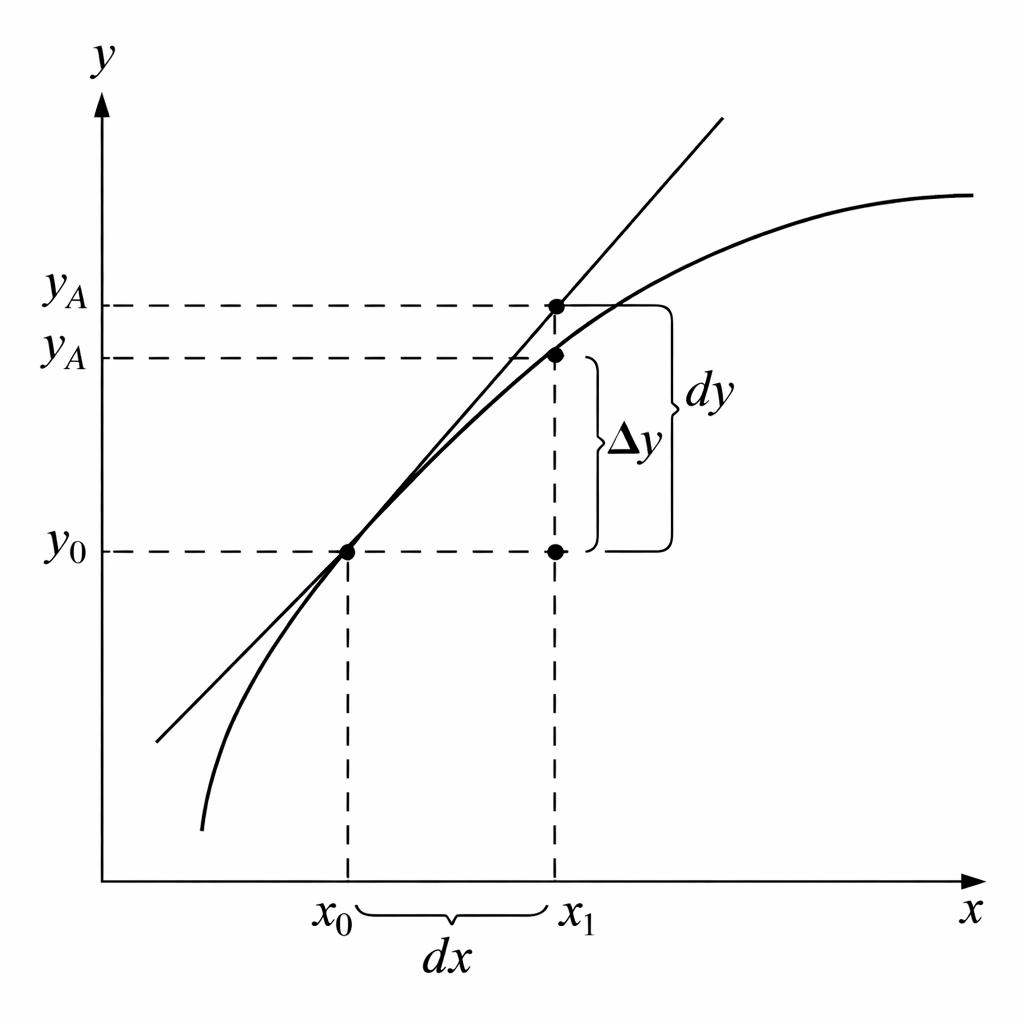
\frac{dy}{dx} = \frac{7x^6}{x^7} = \frac{7}{x}

The Differential¶

Define $dx$ as an arbitrary change in $x$ from its initial value $x_0$ and $dy$ as the resulting change in $y$ along the tangent line from the initial value of the function $y_0 = f(x_0)$ .

The differential of $y=f(x_0)$ evaluated at $x_0$ is

dy = f'(x_0)\, dx.

This represents the change in $y$ along the tangent line at $x_0$ . Graphically, this is shown in Figure 1.

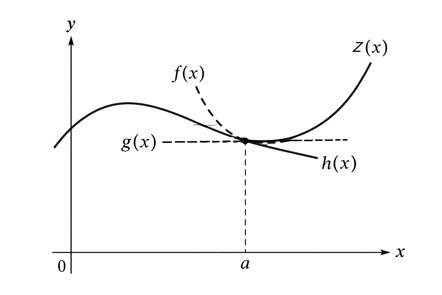
Taylor Series¶

A smooth complex function $z(x)$ can be approximated around $x=a$ by

f(x) = z(a) + z'(a)(x-a) + \frac{1}{2}z''(a)(x-a)^2 + \frac{1}{6}f'''(a)(x-a)^3 + \cdots

This idea underlies many approximation methods in economics.

As shown in Figure 2 a function $z(x)$ being approximated by three different Taylor polynomials (or Taylor series expansions) centered around the point $x=a$ .

The simplest approximation perhaps would simply be $g(x) = a$ . This constant-valued function does not work well, especially if we move away from the point $a$ .

A better approximation would be a linear function of the form $h(x) = z(a) + b(x-a)$ , where $b$ is some slope. But what would be a good value of $b$ ? We saw above that the differential is an equation for the tangent line (or slope) at the point $x = a$ . So, we could argue that the best linear approximation to the function around this point would be

h(x) = z(a) + z'(a)(x-a)

where $z'(a)$ is the derivative of the function evaluated at $x=a$ .

But why stop here? We could improve on this. A better approximation could allow for some curvature. The general form would then be, say, $f(x) = z(a) + z'(a) .(x-a) + c.(x-a)^2$ . Again, we ask, “What would be the best value for $c$ ?” The rate of change of the slope of the quadratic approximation should be equal to the rate of change of change of the function at the $a$ . And since the second derivative of $z(x)$ is $2c$ , then for $f''(x)$ to equal $z''(x)$ at $x = a$ , we need $c = 1/2 z''(a)$ . Hence the quadratic approximation to the function aound $x = a$ is:

f(x) = z(a) + z'(a)(x-a) + \frac{1}{2}f''(a)(x-a)^2

Exteding the above argument for cubic and higher-degree approximations, we could find the $n$ th-degree approximation to the function $z(x)$ , which we could call $m(x)$ , around the point $x = a$ is

m(x) = \frac{z(a)}{0!} + \frac{z'(a)}{1!}(x-a) + \frac{z''(a)}{2!}(x-a)^2 + \cdots + \frac{f^{(n)}(a)}{n!}(x-a)^n

where $f^{(n)}(a)$ is the $n$ the derivative of $z(x)$ evaluated at $x = a$ . The function $m(x)$ above is called the $n$ -th degree Taylor expansion series of $z(x)$ evaluated at $x=a$ .

To sum, $z(x)$ is the original function being approximated (the solid curve). $g(x)$ represents a constant function. $h(x)$ represents the first-order Taylor polynomial, i.e. a straight line that has the same value and slope as $z(x)$ at $x=a$ (or a tangent to $z(x)$ at $x=a$ ). The formula for $f(x)$ is $f(x) = z(a) + z^{\prime }(a)(x-a) + \frac{1}{2} z''(a)(x-a)^2$ representing a second-order (quadratic) polynomial-the dashed curve, which matches better the function’s value, slope, and concavity (curvature) at $x=a$ . It is a better approximation of $z(x)$ near $x=a$ than the linear approximation $h(x)$ and of course the constant function $g(a)$ . The graph demonstrates that as more terms are included in the Taylor polynomial, the approximation of the original function becomes more accurate over a larger range around the center point $x=a$ .

Implicit Differentiation¶

Let’s consider a very simple function,

xy = 7.

Here, possible solutions include $(x,y)=(1,7)$ , $(7,1)$ , and so on.
If we want to find the slope of this function, we can differentiate it.

Finding $y'$

To find $y'$ , we proceed as follows.

(a) We make the main assumption that $y$ is a function of $x$ , i.e. $y=f(x)$ .
We then differentiate both sides of the equation with respect to $x$ .

Hence, we obtain

\frac{d}{dx}[x f(x)] = 0.

Using the product rule, this gives

1\cdot f(x) + x f'(x) = 0.

Equivalently,

y + x y' = 0.

(b) Solving the resulting equation for $y'$ gives

y' = -\frac{y}{x}.

So, if we substitute, for example, $x=1$ and $y=5$ , we obtain the slope of the function at that point:

y' = -5.

Inverse Function Rule for Implicit Functions¶

We can show that

\frac{dy}{dx} = -\frac{f_x}{f_y}.

That is, if we have an implicit function written as

f(x,y) = 0,

then the derivative of $y$ with respect to $x$ can be obtained by:

differentiating $f$ with respect to $x$ to obtain $f_x$ ,
differentiating $f$ with respect to $y$ to obtain $f_y$ ,
taking the ratio $-\dfrac{f_x}{f_y}$ .

This gives the derivative of the implicit function $y$ with respect to $x$ .

It often feels like magic — but it is simply a consequence of the chain rule.

Some Uses of Differentiation in Economics¶

Some common applications of differentiation include:

Increasing and decreasing functions
Relative extrema (maximum or minimum)
Inflection points
Optimization of functions

etc.

A CES production function example¶

Given the CES production function

Q = A\bigl[\alpha K^{-\beta} + (1-\alpha)L^{-\beta}\bigr]^{-1/\beta},

we can show that the elasticity of substitution is constant, as follows.

First-order conditions

The first-order conditions require that

\frac{\partial Q / \partial L}{\partial Q / \partial K} = \frac{P_L}{P_K}.

Using the generalized power function rule, we take the first-order partial derivatives.

For labor,

\frac{\partial Q}{\partial L} = -\frac{1}{\beta} A\bigl[\alpha K^{-\beta} + (1-\alpha)L^{-\beta}\bigr]^{-(1/\beta+1)} (-\beta)(1-\alpha)L^{-\beta-1}.

Canceling the $-\beta$ terms, rearranging $(1-\alpha)$ , and adding the exponents $-(1/\beta)-1$ , we obtain

\frac{\partial Q}{\partial L} = (1-\alpha)A \bigl[\alpha K^{-\beta} + (1-\alpha)L^{-\beta}\bigr]^{-(1+\beta)/\beta} L^{-(1+\beta)}.

Substituting $A^{1+\beta}/A^{\beta}=A$ , we can write

\frac{\partial Q}{\partial L} = (1-\alpha)\frac{A^{1+\beta}}{A^\beta} \bigl[\alpha K^{-\beta} + (1-\alpha)L^{-\beta}\bigr]^{-(1+\beta)/\beta} L^{-(1+\beta)}.

From the CES production function,

A^{1+\beta} \bigl[\alpha K^{-\beta} + (1-\alpha)L^{-\beta}\bigr]^{-(1+\beta)/\beta} = Q^{1+\beta},

and

L^{-(1+\beta)} = \frac{1}{L^{1+\beta}}.

Thus,

\frac{\partial Q}{\partial L} = \frac{1-\alpha}{A^\beta} \left(\frac{Q}{L}\right)^{1+\beta}.

The marginal product of capital

Similarly,

\frac{\partial Q}{\partial K} = \frac{\alpha}{A^\beta} \left(\frac{Q}{K}\right)^{1+\beta}.

Dividing the two equations and equating the result to $P_L/P_K$ (from the FOC) leads to the cancellation of $A^\beta$ and $Q$ :

\frac{1-\alpha}{\alpha} \left(\frac{K}{L}\right)^{1+\beta} = \frac{P_L}{P_K}.

Rearranging,

\left(\frac{K}{L}\right)^{1+\beta} = \frac{\alpha}{1-\alpha} \frac{P_L}{P_K},

and therefore,

\frac{K}{L} = \left(\frac{\alpha}{1-\alpha}\right)^{1/(1+\beta)} \left(\frac{P_L}{P_K}\right)^{1/(1+\beta)}.

Elasticity of substitution

Since $\alpha$ and $\beta$ are constants, we can treat $K/L$ as a function of $P_L/P_K$ .

Let

h = \left(\frac{\alpha}{1-\alpha}\right)^{1/(1+\beta)}.

Then

\frac{K}{L} = h\left(\frac{P_L}{P_K}\right)^{1/(1+\beta)}.

The marginal function is

\frac{d(K/L)}{d(P_L/P_K)} = \frac{h}{1+\beta} \left(\frac{P_L}{P_K}\right)^{1/(1+\beta)-1}.

The average function is

\frac{K/L}{P_L/P_K} = h\left(\frac{P_L}{P_K}\right)^{1/(1+\beta)-1}.

Dividing the marginal function by the average function, we obtain the elasticity of substitution:

\text{MRS} = \frac{d(K/L)}{d(P_L/P_K)} \Big/ \frac{K/L}{P_L/P_K} = \frac{1}{1+\beta}.

This is constant, hence the CES production function exhibits constant elasticity of substitution.

Interpretation

If $-1 < \beta < 0$ , then MRS $> 1$ .
If $\beta = 0$ , then MRS $= 1$ (Cobb–Douglas case).
If $0 < \beta < \infty$ , then MRS $< 1$ .

Footnotes¶

A function need not be defined at the point $a$ in order to have a limit as $x \to a$ . For example,
$f(x) = \frac{x^2 - 1}{x - 1}$
is not defined at $x = 1$ , but
$\lim_{x \to 1} f(x) = 2.$
↩
The two functions discussed above are not continuous. The first is not continuous because $f(a)$ is not defined. The second is not continuous because $f$ does not converge to a limit as $x \to a$ . For example, if
$f(x) = \begin{cases} -1, & x < 0, \\ 1, & x > 0, \end{cases}$
then $f$ has no limit as $x \to 0$ , since the right-hand limit equals 1 while the left-hand limit equals -1.
↩

Basic Differentiation

Functions¶

Graphs¶

Slope¶

Limits¶

Continuity¶

Derivative at a Point¶

Derivative as a Function¶

Second Derivative¶

Basic Rules of Differentiation¶

Constant-function Rule¶

Power-function Rule¶

Generalized Power-function Rule¶

Logarithmic Rule¶

Exponential Rule¶

Sum-difference Rules¶

Product Rule¶

Quotient Rule¶

Chain Rule¶

Chain Rule for Exponential and Logarithmic Functions¶

The general exponential function rule¶

The general natural logarithmic function rule¶

The Differential¶

Taylor Series¶

a. Linear Approximation (n=1n = 1n=1)¶

b. Quadratic Approximation (n=2n = 2n=2)¶

c. Cubic Approximation (n=3n = 3n=3)¶

a. Linear Approximation (n=1n = 1n=1)¶

b. Quadratic Approximation (n=2n = 2n=2)¶

c. Cubic Approximation (n=3n = 3n=3)¶

Implicit Differentiation¶

Inverse Function Rule for Implicit Functions¶

Some Uses of Differentiation in Economics¶

A CES production function example¶

a. Linear Approximation ( $n = 1$ )¶

b. Quadratic Approximation ( $n = 2$ )¶

c. Cubic Approximation ( $n = 3$ )¶

a. Linear Approximation ( $n = 1$ )¶

b. Quadratic Approximation ( $n = 2$ )¶

c. Cubic Approximation ( $n = 3$ )¶