Finding the “best” way to do a specific task in economics often involves what is called an optimization problem .
I — Univariate Optimization ¶ Stationary Points ¶ Generally, we say that x ∗ x^* x ∗ stationary point of a differentiable function f ( x ) f(x) f ( x ) x ∗ x^* x ∗
f ′ ( x ∗ ) = 0. f'(x^*) = 0. f ′ ( x ∗ ) = 0. Necessary First-Order Condition (F.O.C) ¶ More formally, suppose a function f ( x ) f(x) f ( x ) I I I x ∗ x^* x ∗ I I I x = x ∗ x = x^* x = x ∗ f ( x ) f(x) f ( x ) I I I necessary condition is that it is a stationary point for f ( x ) f(x) f ( x ) x = x ∗ x = x^* x = x ∗
f ′ ( x ∗ ) = 0. f'(x^*) = 0. f ′ ( x ∗ ) = 0. Example 1
Let
h ( x ) = − x 2 + 8 x − 15. h(x) = -x^2 + 8x - 15. h ( x ) = − x 2 + 8 x − 15. F.O.C:
− 2 x + 8 = 0. -2x + 8 = 0. − 2 x + 8 = 0. So the stationary point is x ∗ = 4 x^* = 4 x ∗ = 4 y ∗ = 1 y^* = 1 y ∗ = 1
Example 2
Let
z ( x ) = x 2 − 8 x + 17. z(x) = x^2 - 8x + 17. z ( x ) = x 2 − 8 x + 17. F.O.C:
2 x − 8 = 0. 2x - 8 = 0. 2 x − 8 = 0. So the stationary point is x ∗ = 4 x^* = 4 x ∗ = 4 y ∗ = 1 y^* = 1 y ∗ = 1
We have the same stationary point, but clearly these are different functions.
The former is ∩ \cap ∩ ∪ \cup ∪
Sufficient Second-Order Condition (S.O.C) for Maximum/Minimum ¶ Following the two examples above, we can characterize a stationary point as a maximum or minimum by taking the second derivative.
If f ′ ′ ( x ∗ ) < 0 f''(x^*) < 0 f ′′ ( x ∗ ) < 0 maximum .
If f ′ ′ ( x ∗ ) > 0 f''(x^*) > 0 f ′′ ( x ∗ ) > 0 minimum .
Example 1
h ′ ′ ( x ) = − 2. h''(x) = -2. h ′′ ( x ) = − 2. Since this is negative, the stationary point ( 4 , 1 ) (4,1) ( 4 , 1 ) maximum .
Example 2
z ′ ′ ( x ) = 2. z''(x) = 2. z ′′ ( x ) = 2. Since this is positive, the stationary point ( 4 , 1 ) (4,1) ( 4 , 1 ) minimum .
Example 3
Let
p ( x ) = 1 3 x 3 − 1 2 x 2 − 2 x + 20. p(x) = \frac{1}{3}x^3 - \frac{1}{2}x^2 - 2x + 20. p ( x ) = 3 1 x 3 − 2 1 x 2 − 2 x + 20. The F.O.C gives
p ′ ( x ) = x 2 − x − 2 = 0 , p'(x) = x^2 - x - 2 = 0, p ′ ( x ) = x 2 − x − 2 = 0 , which implies x ∗ = − 1 x^* = -1 x ∗ = − 1 x ∗ = 2 x^* = 2 x ∗ = 2
The S.O.C gives
p ′ ′ ( x ) = 2 x − 1. p''(x) = 2x - 1. p ′′ ( x ) = 2 x − 1. At x ∗ = − 1 x^* = -1 x ∗ = − 1 p ′ ′ ( − 1 ) = − 3 < 0 p''(-1) = -3 < 0 p ′′ ( − 1 ) = − 3 < 0 maximum
At x ∗ = 2 x^* = 2 x ∗ = 2 p ′ ′ ( 2 ) = 3 > 0 p''(2) = 3 > 0 p ′′ ( 2 ) = 3 > 0 minimum
S.O.C Is Sufficient but Not Necessary ¶ Consider
The F.O.C gives x ∗ = 0 x^* = 0 x ∗ = 0
The S.O.C also gives 0, which is neither positive nor negative.
Yet, x ∗ = 0 x^* = 0 x ∗ = 0 minimum .
Global and Local Minimum/Maximum ¶ We must distinguish between global and local extrema.
Global Maximum ¶ If f ( x ) f(x) f ( x ) x ∗ x^* x ∗ x ∗ x^* x ∗ global maximum if
f ′ ( x ) ≥ 0 for all x ≤ x ∗ , and f ′ ( x ) ≤ 0 for all x ≥ x ∗ . f'(x) \ge 0 \text{ for all } x \le x^*,
\quad \text{and} \quad
f'(x) \le 0 \text{ for all } x \ge x^*. f ′ ( x ) ≥ 0 for all x ≤ x ∗ , and f ′ ( x ) ≤ 0 for all x ≥ x ∗ . That is, the function increases up to x ∗ x^* x ∗
Global Minimum ¶ Similarly, x ∗ x^* x ∗ global minimum if
f ′ ( x ) ≤ 0 for all x ≤ x ∗ , and f ′ ( x ) ≥ 0 for all x ≥ x ∗ . f'(x) \le 0 \text{ for all } x \le x^*,
\quad \text{and} \quad
f'(x) \ge 0 \text{ for all } x \ge x^*. f ′ ( x ) ≤ 0 for all x ≤ x ∗ , and f ′ ( x ) ≥ 0 for all x ≥ x ∗ . Local Maximum / Minimum ¶ We speak of a local maximum or minimum if x ∗ x^* x ∗ only in a neighborhood of x ∗ x^* x ∗ , not over the entire domain.
Concavity and Convexity ¶ If f ( x ) f(x) f ( x ) strictly concave on ( m , n ) (m,n) ( m , n ) x ∗ x^* x ∗ m < x ∗ < n m < x^* < n m < x ∗ < n x ∗ x^* x ∗ local maximum .
If f ( x ) f(x) f ( x ) global maximum .
Conversely,
If f ( x ) f(x) f ( x ) strictly convex on ( m , n ) (m,n) ( m , n ) x ∗ x^* x ∗ x ∗ x^* x ∗ local minimum .
If f ( x ) f(x) f ( x ) global minimum .
Inflection Points ¶ Consider the function
k ( x ) = 1 + ( x − 4 ) 3 . k(x) = 1 + (x - 4)^3. k ( x ) = 1 + ( x − 4 ) 3 . The F.O.C gives a stationary point ( 4 , 1 ) (4,1) ( 4 , 1 )
The S.O.C evaluated at this point is 0, so it is inconclusive.
We must then take higher-order derivatives.
If the first nonzero higher-order derivative evaluated at the stationary point is:
If the first non-zero derivative at the stationary point c c c even order (n = 2 , 4 , 6... n = 2, 4, 6... n = 2 , 4 , 6...
Derivative Sign Result Visual Intuition f ( n ) ( c ) > 0 f^{(n)}(c) > 0 f ( n ) ( c ) > 0 Local Minimum The function “curves up” away from the point in all directions. f ( n ) ( c ) < 0 f^{(n)}(c) < 0 f ( n ) ( c ) < 0 Local Maximum The function “curves down” away from the point in all directions.
For this example,
k ′ ′ ′ ( 4 ) ≠ 0 , k'''(4) \ne 0, k ′′′ ( 4 ) = 0 , which is the third (odd) derivative.
Hence, ( 4 , 1 ) (4,1) ( 4 , 1 ) inflection point .
Stationary Points and Higher-Order Derivative Test
Find the stationary points of the following functions and determine whether you have a minimum, maximum, or inflection point by determining whether at the stationary point the function is convex or concave (or neither).
(i) f ( x ) = − x 3 + 6 x 2 + 15 x − 32 f(x) = -x^3 + 6x^2 + 15x - 32 f ( x ) = − x 3 + 6 x 2 + 15 x − 32
(ii) f ( x ) = ( 2 x − 7 ) 3 f(x) = (2x - 7)^3 f ( x ) = ( 2 x − 7 ) 3
(iii) f ( x ) = ( x + 2 ) 4 f(x) = (x + 2)^4 f ( x ) = ( x + 2 ) 4
(iv) f ( x ) = − 2 ( x − 6 ) 6 f(x) = -2(x - 6)^6 f ( x ) = − 2 ( x − 6 ) 6
(v) f ( x ) = x 4 f(x) = x^4 f ( x ) = x 4
Answers
(i) f ′ ( x ) = − 3 x 2 + 12 x + 15 f'(x) = -3x^2 + 12x + 15 f ′ ( x ) = − 3 x 2 + 12 x + 15
Setting f ′ ( x ) = 0 f'(x)=0 f ′ ( x ) = 0
x = − 1 and x = 5 x = -1 \quad \text{and} \quad x = 5 x = − 1 and x = 5 Second derivative:
f ′ ′ ( x ) = − 6 x + 12 f''(x) = -6x + 12 f ′′ ( x ) = − 6 x + 12 f ′ ′ ( − 1 ) = 18 > 0 ⇒ minimum f''(-1) = 18 > 0 \Rightarrow \text{minimum} f ′′ ( − 1 ) = 18 > 0 ⇒ minimum f ′ ′ ( 5 ) = − 18 < 0 ⇒ maximum f''(5) = -18 < 0 \Rightarrow \text{maximum} f ′′ ( 5 ) = − 18 < 0 ⇒ maximum Inflection point:
f ′ ′ ( x ) = 0 ⇒ x = 2 f''(x)=0 \Rightarrow x=2 f ′′ ( x ) = 0 ⇒ x = 2 (ii) f ′ ( x ) = 6 ( 2 x − 7 ) 2 f'(x) = 6(2x - 7)^2 f ′ ( x ) = 6 ( 2 x − 7 ) 2
Hence, x = 3.5 \text{Hence, }x = 3.5 Hence, x = 3.5 f ′ ′ ( x ) = 24 ( 2 x − 7 ) f''(x) = 24(2x - 7) f ′′ ( x ) = 24 ( 2 x − 7 ) f ′ ′ ( 3.5 ) = 0 f''(3.5) = 0 f ′′ ( 3.5 ) = 0 f ′ ′ ′ ( x ) = 48 f'''(x) = 48 f ′′′ ( x ) = 48 Since the first nonzero derivative at the critical point is of odd order , we have an inflection point at x = 3.5 x=3.5 x = 3.5
(iii) f ′ ( x ) = 4 ( x + 2 ) 3 f'(x) = 4(x+2)^3 f ′ ( x ) = 4 ( x + 2 ) 3
f ′ ′ ( − 2 ) = 0 , f ′ ′ ′ ( − 2 ) = 0 , f ( 4 ) ( − 2 ) = 24 > 0 f''(-2)=0, \quad f'''(-2)=0, \quad f^{(4)}(-2)=24>0 f ′′ ( − 2 ) = 0 , f ′′′ ( − 2 ) = 0 , f ( 4 ) ( − 2 ) = 24 > 0 The first nonzero derivative is even and positive , hence we have a minimum .
(iv) f ′ ( x ) = − 12 ( x − 6 ) 5 f'(x) = -12(x-6)^5 f ′ ( x ) = − 12 ( x − 6 ) 5
All derivatives up to order 5 vanish.
f ( 6 ) ( 6 ) = − 1440 < 0 f^{(6)}(6) = -1440 < 0 f ( 6 ) ( 6 ) = − 1440 < 0 The first nonzero derivative is even and negative , hence we have a maximum .
(v) f ′ ( x ) = 4 x 3 f'(x) = 4x^3 f ′ ( x ) = 4 x 3
All derivatives up to order 3 vanish.
f ( 0 ) ( 4 ) = 24 > 0 f^{(0)}(4) = 24 > 0 f ( 0 ) ( 4 ) = 24 > 0 The first nonzero derivative is of even order and it’s value is positive, hence we have an local minimum .
Economic Applications ¶ A Monopolist’s Optimal Pricing Scheme
Strategic Behavior of Duopolists
Rules versus Discretion in Monetary Policy
The Inflation Tax and Seigniorage
The Golden Rule
II — Multivariate Optimization ¶ We now generalize the univariate techniques to multivariate optimization.
Multivariate First-Order Condition ¶ If we have a function
y = f ( x 1 , x 2 , … , x n ) y = f(x_1, x_2, \ldots, x_n) y = f ( x 1 , x 2 , … , x n ) that is differentiable with respect to each of its arguments and has a stationary point at
( x 1 ∗ , x 2 ∗ , … , x n ∗ ) (x_1^*, x_2^*, \ldots, x_n^*) ( x 1 ∗ , x 2 ∗ , … , x n ∗ )
That is,
f 1 ( x 1 ∗ , x 2 ∗ , … , x n ∗ ) = 0 f 2 ( x 1 ∗ , x 2 ∗ , … , x n ∗ ) = 0 ⋮ f n ( x 1 ∗ , x 2 ∗ , … , x n ∗ ) = 0 f_1(x_1^*, x_2^*, \ldots, x_n^*) = 0 \\
f_2(x_1^*, x_2^*, \ldots, x_n^*) = 0 \\
\vdots \\
f_n(x_1^*, x_2^*, \ldots, x_n^*) = 0 f 1 ( x 1 ∗ , x 2 ∗ , … , x n ∗ ) = 0 f 2 ( x 1 ∗ , x 2 ∗ , … , x n ∗ ) = 0 ⋮ f n ( x 1 ∗ , x 2 ∗ , … , x n ∗ ) = 0 Example 1
Consider the bivariate function
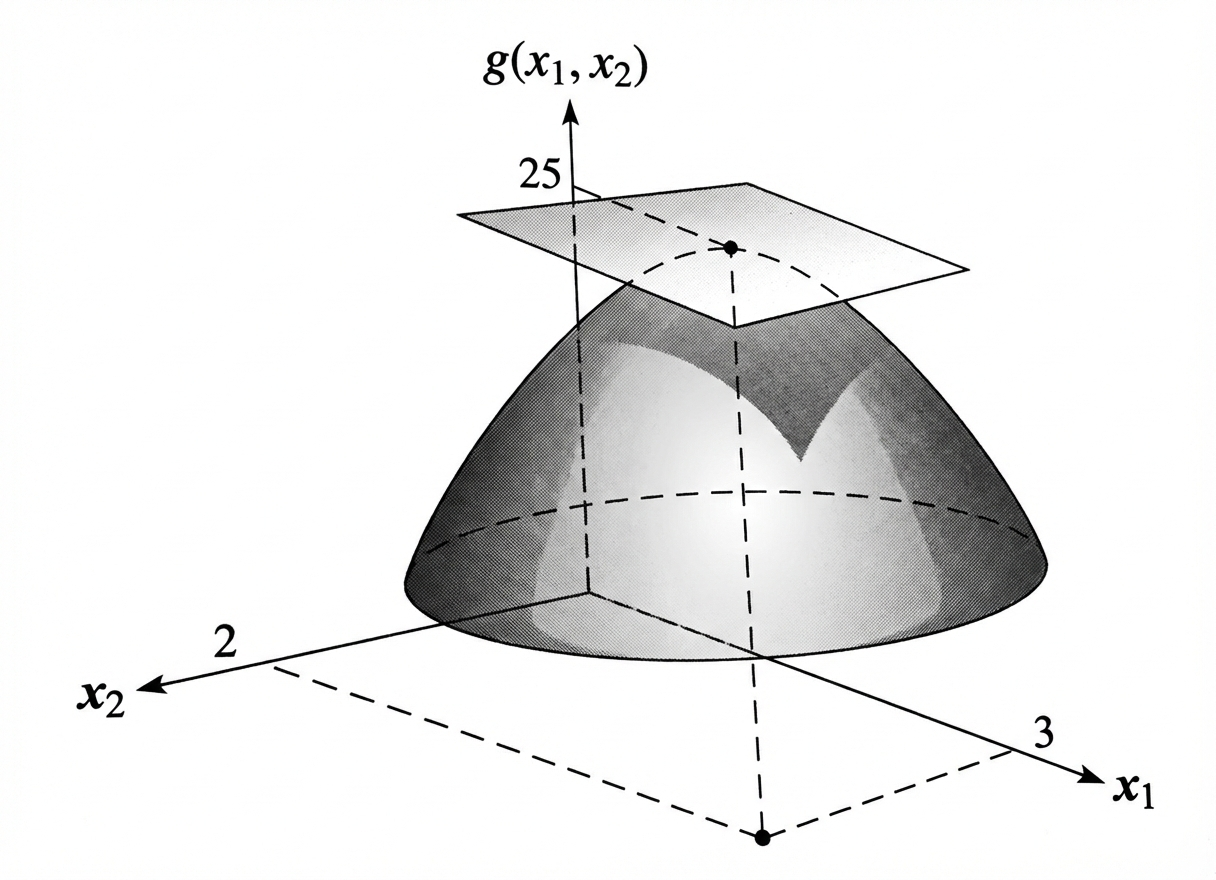
g ( x 1 , x 2 ) = 6 x 1 − x 1 2 + 16 x 2 − 4 x 2 2 g(x_1, x_2) = 6x_1 - x_1^2 + 16x_2 - 4x_2^2 g ( x 1 , x 2 ) = 6 x 1 − x 1 2 + 16 x 2 − 4 x 2 2 The first-order conditions are
g 1 ( x 1 , x 2 ) = 6 − 2 x 1 = 0 g 2 ( x 1 , x 2 ) = 16 − 8 x 2 = 0 g_1(x_1, x_2) = 6 - 2x_1 = 0 \\
g_2(x_1, x_2) = 16 - 8x_2 = 0 g 1 ( x 1 , x 2 ) = 6 − 2 x 1 = 0 g 2 ( x 1 , x 2 ) = 16 − 8 x 2 = 0 The single stationary point is therefore
x 1 ∗ = 3 , x 2 ∗ = 2 x_1^* = 3, \quad x_2^* = 2 x 1 ∗ = 3 , x 2 ∗ = 2 and the value of the function at this point is
g ( 3 , 2 ) = 25. g(3,2) = 25. g ( 3 , 2 ) = 25. We will show later using the second-order condition that this stationary point represents a maximum .
Let’s visualize the equation and its stationary point.
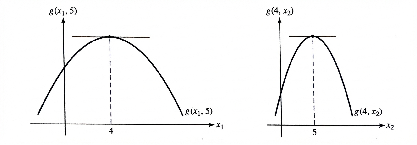
If we take a slice of the function g ( x 1 , x 2 ) g(x_1, x_2) g ( x 1 , x 2 ) x 2 = 2 x_2 = 2 x 2 = 2 x 1 = 3 x_1 = 3 x 1 = 3 x 1 = 3 x_1 = 3 x 1 = 3 x 2 = 2 x_2 = 2 x 2 = 2
Example 2
Consider the function
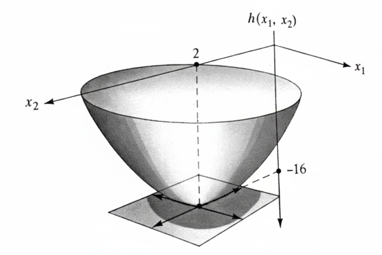
h ( x 1 , x 2 ) = x 1 2 + 4 x 2 2 − 2 x 1 − 16 x 2 + x 1 x 2 h(x_1, x_2) = x_1^2 + 4x_2^2 - 2x_1 - 16x_2 + x_1 x_2 h ( x 1 , x 2 ) = x 1 2 + 4 x 2 2 − 2 x 1 − 16 x 2 + x 1 x 2 The first-order conditions give
h 1 ( x 1 , x 2 ) = 2 x 1 − 2 + x 2 = 0 h 2 ( x 1 , x 2 ) = 8 x 2 − 16 + x 1 = 0 h_1(x_1, x_2) = 2x_1 - 2 + x_2 = 0 \\
h_2(x_1, x_2) = 8x_2 - 16 + x_1 = 0 h 1 ( x 1 , x 2 ) = 2 x 1 − 2 + x 2 = 0 h 2 ( x 1 , x 2 ) = 8 x 2 − 16 + x 1 = 0 Hence the single stationary point is
x 1 ∗ = 0 , x 2 ∗ = 2 x_1^* = 0, \quad x_2^* = 2 x 1 ∗ = 0 , x 2 ∗ = 2 and the value of the function at this point is
h ( 0 , 2 ) = − 16. h(0,2) = -16. h ( 0 , 2 ) = − 16. Below is a visualization of this function with the plane tangent and stationary point.
Second-Order Condition in the Bivariate Case ¶ For the univariate case, the second differential of a function can be considered as the differential of the first differential and denoted as
d ( d y ) = d 2 y . d(dy) = d^2 y. d ( d y ) = d 2 y . For y = f ( x ) y = f(x) y = f ( x )
d 2 y = f ′ ′ ( x ) ( d x ) 2 , d^2 y = f''(x)(dx)^2, d 2 y = f ′′ ( x ) ( d x ) 2 , which is nonnegative for any d x dx d x
Second Differential in the Bivariate Case ¶ For a bivariate function y = f ( x 1 , x 2 ) y = f(x_1, x_2) y = f ( x 1 , x 2 )
d y = f 1 ( x 1 , x 2 ) , d x 1 + f 2 ( x 1 , x 2 ) , d x 2 . dy = f_1(x_1, x_2),dx_1 + f_2(x_1, x_2),dx_2. d y = f 1 ( x 1 , x 2 ) , d x 1 + f 2 ( x 1 , x 2 ) , d x 2 . Taking the total derivative of this expression yields the second total differential:
d 2 y = f 11 ( d x 1 ) 2 + f 22 ( d x 2 ) 2 + 2 f 12 d x 1 d x 2 . d^2 y
= f_{11}(dx_1)^2 + f_{22}(dx_2)^2 + 2f_{12}dx_1 dx_2. d 2 y = f 11 ( d x 1 ) 2 + f 22 ( d x 2 ) 2 + 2 f 12 d x 1 d x 2 . Sufficient Conditions for Local Maxima and Minima ¶ If d 2 y < 0 d^2 y < 0 d 2 y < 0 ( d x 1 , d x 2 ) (dx_1, dx_2) ( d x 1 , d x 2 ) local maximum .
If d 2 y > 0 d^2 y > 0 d 2 y > 0 ( d x 1 , d x 2 ) (dx_1, dx_2) ( d x 1 , d x 2 ) local minimum .
A necessary condition for a minimum is
f 11 > 0 and f 22 > 0 , f_{11} > 0 \quad \text{and} \quad f_{22} > 0, f 11 > 0 and f 22 > 0 , and for a maximum,
f 11 < 0 and f 22 < 0. f_{11} < 0 \quad \text{and} \quad f_{22} < 0. f 11 < 0 and f 22 < 0. However, the cross-partial derivative f 12 f_{12} f 12
Completing the Square ¶ By completing the square, the second differential can be rewritten, leading to the condition:
f 11 f 22 > ( f 12 ) 2 . f_{11} f_{22} > (f_{12})^2. f 11 f 22 > ( f 12 ) 2 . Second-Order Condition for a Maximum ¶ If y = f ( x 1 , x 2 ) y = f(x_1, x_2) y = f ( x 1 , x 2 ) ( x 1 ∗ , x 2 ∗ ) (x_1^*, x_2^*) ( x 1 ∗ , x 2 ∗ )
f 11 ( x 1 ∗ , x 2 ∗ ) < 0 and f 11 f 22 > ( f 12 ) 2 , f_{11}(x_1^*, x_2^*) < 0
\quad \text{and} \quad
f_{11} f_{22} > (f_{12})^2, f 11 ( x 1 ∗ , x 2 ∗ ) < 0 and f 11 f 22 > ( f 12 ) 2 , then the function reaches a maximum at that point.
Second-Order Condition for a Minimum ¶ If
f 11 ( x 1 ∗ , x 2 ∗ ) > 0 and f 11 f 22 > ( f 12 ) 2 , f_{11}(x_1^*, x_2^*) > 0
\quad \text{and} \quad
f_{11} f_{22} > (f_{12})^2, f 11 ( x 1 ∗ , x 2 ∗ ) > 0 and f 11 f 22 > ( f 12 ) 2 , then the function reaches a minimum .
If f 11 f 22 < ( f 12 ) 2 f_{11} f_{22} < (f_{12})^2 f 11 f 22 < ( f 12 ) 2 saddle point .
If f 11 f 22 = ( f 12 ) 2 f_{11} f_{22} = (f_{12})^2 f 11 f 22 = ( f 12 ) 2 inconclusive .
Let’s continue with the example above.
The second partial derivatives of
h ( x 1 , x 2 ) = x 1 2 + 4 x 2 2 − 2 x 1 − 16 x 2 + x 1 x 2 h(x_1,x_2) = x_1^2 + 4x_2^2 - 2x_1 - 16x_2 + x_1x_2 h ( x 1 , x 2 ) = x 1 2 + 4 x 2 2 − 2 x 1 − 16 x 2 + x 1 x 2 are
h 11 ( x 1 , x 2 ) = 2 and h 22 ( x 1 , x 2 ) = 8 h_{11}(x_1,x_2) = 2 \quad \text{and} \quad h_{22}(x_1,x_2) = 8 h 11 ( x 1 , x 2 ) = 2 and h 22 ( x 1 , x 2 ) = 8 Both are positive. The cross-partial derivative is
h 12 ( x 1 , x 2 ) = 1. h_{12}(x_1,x_2) = 1. h 12 ( x 1 , x 2 ) = 1. Since
h 11 h 22 > ( h 12 ) 2 , h_{11} h_{22} > (h_{12})^2, h 11 h 22 > ( h 12 ) 2 , that is,
the stationary point ( 0 , 2 ) (0,2) ( 0 , 2 ) minimum .
As another example, consider
g ( x 1 , x 2 ) = 6 x 1 − x 1 2 + 16 x 2 − 4 x 2 2 . g(x_1,x_2) = 6x_1 - x_1^2 + 16x_2 - 4x_2^2. g ( x 1 , x 2 ) = 6 x 1 − x 1 2 + 16 x 2 − 4 x 2 2 . The second partial derivatives are
g 11 ( x 1 , x 2 ) = − 2 and g 22 ( x 1 , x 2 ) = − 8 , g_{11}(x_1,x_2) = -2 \quad \text{and} \quad g_{22}(x_1,x_2) = -8, g 11 ( x 1 , x 2 ) = − 2 and g 22 ( x 1 , x 2 ) = − 8 , and the cross-partial derivative is
g 12 ( x 1 , x 2 ) = 0. g_{12}(x_1,x_2) = 0. g 12 ( x 1 , x 2 ) = 0. Since the second partial derivatives are both negative and
g 11 g 22 > ( g 12 ) 2 , g_{11} g_{22} > (g_{12})^2, g 11 g 22 > ( g 12 ) 2 , that is,
we have the conditions for a maximum .
Second-Order Condition in the General Multivariate Case ¶ Let us use the tools of matrix algebra to develop a set of conditions that enables us to find the sign of the second total differential of a multivariate function.
First, assume a bivariate case for which the second total differential is given by
d 2 y = f 11 ( d x 1 ) 2 + f 22 ( d x 2 ) 2 + 2 f 12 ( d x 1 ) ( d x 2 ) . d^2 y
=
f_{11}(dx_1)^2
+
f_{22}(dx_2)^2
+
2 f_{12}(dx_1)(dx_2). d 2 y = f 11 ( d x 1 ) 2 + f 22 ( d x 2 ) 2 + 2 f 12 ( d x 1 ) ( d x 2 ) . This expression can be written in matrix form as the quadratic form of the two variables d x 1 dx_1 d x 1 d x 2 dx_2 d x 2
d 2 y = [ d x 1 d x 2 ] [ f 11 f 12 f 21 f 22 ] [ d x 1 d x 2 ] . d^2 y
=
\begin{bmatrix}
dx_1 & dx_2
\end{bmatrix}
\begin{bmatrix}
f_{11} & f_{12} \\
f_{21} & f_{22}
\end{bmatrix}
\begin{bmatrix}
dx_1 \\
dx_2
\end{bmatrix}. d 2 y = [ d x 1 d x 2 ] [ f 11 f 21 f 12 f 22 ] [ d x 1 d x 2 ] . In other words, the second total differential (or second total derivative) for a multivariate function can be written more generally as
d 2 y = d x ′ H d x = [ d x 1 d x 2 ⋯ d x n ] [ f 11 f 12 ⋯ f 1 n f 21 f 22 ⋯ f 2 n ⋮ ⋮ ⋱ ⋮ f n 1 f n 2 ⋯ f n n ] [ d x 1 d x 2 ⋮ d x n ] . d^2 y
=
dx' H dx
=
\begin{bmatrix}
dx_1 & dx_2 & \cdots & dx_n
\end{bmatrix}
\begin{bmatrix}
f_{11} & f_{12} & \cdots & f_{1n} \\
f_{21} & f_{22} & \cdots & f_{2n} \\
\vdots & \vdots & \ddots & \vdots \\
f_{n1} & f_{n2} & \cdots & f_{nn}
\end{bmatrix}
\begin{bmatrix}
dx_1 \\
dx_2 \\
\vdots \\
dx_n
\end{bmatrix}. d 2 y = d x ′ H d x = [ d x 1 d x 2 ⋯ d x n ] ⎣ ⎡ f 11 f 21 ⋮ f n 1 f 12 f 22 ⋮ f n 2 ⋯ ⋯ ⋱ ⋯ f 1 n f 2 n ⋮ f nn ⎦ ⎤ ⎣ ⎡ d x 1 d x 2 ⋮ d x n ⎦ ⎤ . Here, H H H Hessian matrix , and d x dx d x
All that remains is to determine the sign definiteness of the quadratic form by determining the sign definiteness of the Hessian.
Interpreting the Second-Order Condition ¶ The sign of the second total differential d 2 y d^2 y d 2 y
Because
d 2 y = d x ′ H d x , d^2 y = dx' H dx, d 2 y = d x ′ H d x , the problem reduces to determining the sign definiteness of the Hessian matrix H H H .
Positive and Negative Definiteness ¶ These cases correspond to the curvature of the function at a critical point.
Second-Order Conditions for Optimization ¶ Suppose y = f ( x 1 , … , x n ) y = f(x_1, \ldots, x_n) y = f ( x 1 , … , x n ) ∇ f = 0 \nabla f = 0 ∇ f = 0 x ∗ x^* x ∗
If H ( x ∗ ) H(x^*) H ( x ∗ ) negative definite , then x ∗ x^* x ∗ local maximum .
If H ( x ∗ ) H(x^*) H ( x ∗ ) positive definite , then x ∗ x^* x ∗ local minimum .
If H ( x ∗ ) H(x^*) H ( x ∗ ) indefinite , then x ∗ x^* x ∗ saddle point .
• In one variable , if the first nonzero derivative at a stationary point is of odd order , the point is an inflection point .
• In multiple variables , if the Hessian is indefinite (determinant < 0), the stationary point is a saddle point .
An inflection point concerns curvature along a single line. A saddle point concerns curvature across different directions.
Sylvester’s Criterion (Practical Test) ¶ In practice, definiteness is checked using principal minors of the Hessian.
Bivariate Case (n = 2 n = 2 n = 2 ¶ Let
H = [ f 11 f 12 f 21 f 22 ] . H =
\begin{bmatrix}
f_{11} & f_{12} \\
f_{21} & f_{22}
\end{bmatrix}. H = [ f 11 f 21 f 12 f 22 ] . Then:
H H H positive definite if
f 11 > 0 f_{11} > 0 f 11 > 0 det ( H ) > 0 \det(H) > 0 det ( H ) > 0
H H H negative definite if
f 11 < 0 f_{11} < 0 f 11 < 0 det ( H ) > 0 \det(H) > 0 det ( H ) > 0
H H H indefinite if
det ( H ) < 0 \det(H) < 0 det ( H ) < 0
This criterion is widely used in economics because it avoids computing the quadratic form directly.
Example
Consider the function
y = − x 1 2 − 2 x 2 2 + 4 x 1 x 2 . y = -x_1^2 - 2x_2^2 + 4x_1 x_2. y = − x 1 2 − 2 x 2 2 + 4 x 1 x 2 . The Hessian matrix is
H = [ − 2 4 4 − 4 ] . H =
\begin{bmatrix}
-2 & 4 \\
4 & -4
\end{bmatrix}. H = [ − 2 4 4 − 4 ] . Compute the determinant:
det ( H ) = ( − 2 ) ( − 4 ) − 16 = − 8 < 0. \det(H) = (-2)(-4) - 16 = -8 < 0. det ( H ) = ( − 2 ) ( − 4 ) − 16 = − 8 < 0. Since the determinant is negative, the Hessian is indefinite , and the critical point is a saddle point .
Economic Interpretation ¶ Concavity (negative definite Hessian) corresponds to diminishing marginal returns and guarantees interior maxima in optimization problems.
Convexity (positive definite Hessian) corresponds to cost minimization problems.
Indefiniteness indicates instability or saddle behavior, common in strategic or general equilibrium settings.
The second-order condition in multivariate optimization reduces to checking the sign definiteness of the Hessian matrix .
Matrix algebra provides a compact and powerful way to characterize curvature, stability, and optimality in economic models.
Optimizing Multivariate Functions ¶ The Hessian Test Procedure
To classify a stationary point ( x , y ) (x, y) ( x , y ) f ( x , y ) f(x, y) f ( x , y )
Find Stationary Points: Set first partial derivatives to zero: f x = 0 f_x = 0 f x = 0 f y = 0 f_y = 0 f y = 0
Calculate the Hessian Matrix (H H H
H = [ f x x f x y f y x f y y ] H = \begin{bmatrix} f_{xx} & f_{xy} \\ f_{yx} & f_{yy} \end{bmatrix} H = [ f xx f y x f x y f yy ] Evaluate the Determinant (D D D
D = f x x f y y − ( f x y ) 2 D = f_{xx} f_{yy} - (f_{xy})^2 D = f xx f yy − ( f x y ) 2 Classification Rules:
If D > 0 D > 0 D > 0 f x x > 0 f_{xx} > 0 f xx > 0 Local Minimum
If D > 0 D > 0 D > 0 f x x < 0 f_{xx} < 0 f xx < 0 Local Maximum
If D < 0 D < 0 D < 0 Saddle Point
If D = 0 D = 0 D = 0 Inconclusive
Worked Solutions
i. f ( x , y ) = 3 x 2 − x y + 2 y 2 − 4 x − 7 y + 12 f(x,y) = 3x^2 - xy + 2y^2 - 4x - 7y + 12 f ( x , y ) = 3 x 2 − x y + 2 y 2 − 4 x − 7 y + 12 ¶ a. Find Stationary Points
Solving the system:
From f y f_y f y x = 4 y − 7 x = 4y - 7 x = 4 y − 7 f x f_x f x 6 ( 4 y − 7 ) − y − 4 = 0 6(4y - 7) - y - 4 = 0 6 ( 4 y − 7 ) − y − 4 = 0 24 y − 42 − y − 4 = 0 ⟹ 23 y = 46 ⟹ y = 2 24y - 42 - y - 4 = 0 \implies 23y = 46 \implies \mathbf{y = 2} 24 y − 42 − y − 4 = 0 ⟹ 23 y = 46 ⟹ y = 2 x = 4 ( 2 ) − 7 ⟹ x = 1 x = 4(2) - 7 \implies \mathbf{x = 1} x = 4 ( 2 ) − 7 ⟹ x = 1
Note that you can actually use x = A − 1 b x=A^{-1}b x = A − 1 b
b. Hessian Classification
Conclusion: Since D > 0 D > 0 D > 0 f x x > 0 f_{xx} > 0 f xx > 0 ( 1 , 2 ) (1, 2) ( 1 , 2 )
ii. f ( x , y ) = 60 x + 34 y − 4 x y − 6 x 2 − 3 y 2 + 5 f(x, y) = 60x + 34y - 4xy - 6x^2 - 3y^2 + 5 f ( x , y ) = 60 x + 34 y − 4 x y − 6 x 2 − 3 y 2 + 5 ¶ a. Find Stationary Points
Solving the system:
Multiply first equation by 3: 9 x + 3 y = 45 9x + 3y = 45 9 x + 3 y = 45 ( 9 x − 2 x ) = 45 − 17 ⟹ 7 x = 28 ⟹ x = 4 (9x - 2x) = 45 - 17 \implies 7x = 28 \implies \mathbf{x = 4} ( 9 x − 2 x ) = 45 − 17 ⟹ 7 x = 28 ⟹ x = 4 3 ( 4 ) + y = 15 ⟹ y = 3 3(4) + y = 15 \implies \mathbf{y = 3} 3 ( 4 ) + y = 15 ⟹ y = 3
b. Hessian Classification
Conclusion: Since D > 0 D > 0 D > 0 f x x < 0 f_{xx} < 0 f xx < 0 ( 4 , 3 ) (4, 3) ( 4 , 3 )
iii. f ( x , y ) = 48 y − 3 x 2 − 6 x y − 2 y 2 + 72 x f(x,y) = 48y - 3x^2 - 6xy - 2y^2 + 72x f ( x , y ) = 48 y − 3 x 2 − 6 x y − 2 y 2 + 72 x ¶ a. Find Stationary Points
Solving the system:
From first eq, x = 12 − y x = 12 - y x = 12 − y 3 ( 12 − y ) + 2 y = 24 ⟹ 36 − 3 y + 2 y = 24 ⟹ − y = − 12 ⟹ y = 12 3(12 - y) + 2y = 24 \implies 36 - 3y + 2y = 24 \implies -y = -12 \implies \mathbf{y = 12} 3 ( 12 − y ) + 2 y = 24 ⟹ 36 − 3 y + 2 y = 24 ⟹ − y = − 12 ⟹ y = 12 x = 0 \mathbf{x = 0} x = 0
b. Hessian Classification
Conclusion: Since D < 0 D < 0 D < 0 ( 0 , 12 ) (0, 12) ( 0 , 12 )
iv. f ( x , y ) = 5 x 2 − 3 y 2 − 30 x + 7 y + 4 x y f(x, y) = 5x^2 - 3y^2 - 30x + 7y + 4xy f ( x , y ) = 5 x 2 − 3 y 2 − 30 x + 7 y + 4 x y ¶ a. Find Stationary Points
Hence, x = 2 , y = 2.5 x = 2, y = 2.5 x = 2 , y = 2.5
b. Hessian Classification
Conclusion: Since D < 0 D < 0 D < 0 saddle point .
v. f ( x , y ) = x 3 − 3 x + y 2 − 4 y f(x,y) = x^3 - 3x + y^2 - 4y f ( x , y ) = x 3 − 3 x + y 2 − 4 y ¶ a. Find Stationary Points
Compute the partial derivatives.
Set both equal to zero.
From f x = 0 f_{x}=0 f x = 0
3 x 2 − 3 = 0 ⇒ x 2 = 1 ⇒ x = ± 1. 3x^2 - 3 = 0
\quad\Rightarrow\quad
x^2 = 1
\quad\Rightarrow\quad
x = \pm 1. 3 x 2 − 3 = 0 ⇒ x 2 = 1 ⇒ x = ± 1. From f x 2 = 0 f_{x_2}=0 f x 2 = 0
2 y − 4 = 0 ⇒ y = 2. 2y - 4 = 0
\quad\Rightarrow\quad
y = 2. 2 y − 4 = 0 ⇒ y = 2. We therefore have two critical points:
( 1 , 2 ) and ( − 1 , 2 ) . (1,2)
\quad\text{and}\quad
(-1,2). ( 1 , 2 ) and ( − 1 , 2 ) . Both are integers — nice and clean.
b. Hessian Classification
Compute the second partial derivatives.
The Hessian matrix is
H = [ 6 x 0 0 2 ] . H =
\begin{bmatrix}
6x & 0 \\
0 & 2
\end{bmatrix}. H = [ 6 x 0 0 2 ] . Note that the determinant is
∣ H ∣ = ( 6 x ) ( 2 ) − 0 = 12 x . |H| = (6x)(2) - 0 = 12x. ∣ H ∣ = ( 6 x ) ( 2 ) − 0 = 12 x . Classification
At ( 1 , 2 ) (1,2) ( 1 , 2 )
∣ H 1 ∣ = 6 > 0 / / ∣ H 2 ∣ = ∣ H ∣ = 12 ( 1 ) = 12 > 0 |H_1| = 6 > 0 //
|H_2| = |H| = 12(1) = 12 > 0 ∣ H 1 ∣ = 6 > 0//∣ H 2 ∣ = ∣ H ∣ = 12 ( 1 ) = 12 > 0 So the Hessian is positive definite .
⇒ Local minimum at ( 1 , 2 ) .
\Rightarrow
\textbf{Local minimum at } (1,2). ⇒ Local minimum at ( 1 , 2 ) .
At ( − 1 , 2 ) (-1,2) ( − 1 , 2 )
∣ H 2 ∣ = 12 ( − 1 ) = − 12 < 0. |H_2| = 12(-1) = -12 < 0. ∣ H 2 ∣ = 12 ( − 1 ) = − 12 < 0. Since the determinant is negative, the Hessian is sign indefinite .
⇒ Saddle point at ( − 1 , 2 ) .
\Rightarrow
\textbf{Saddle point at } (-1,2). ⇒ Saddle point at ( − 1 , 2 ) .
Final Answer
( 1 , 2 ) (1,2) ( 1 , 2 ) local minimum
( − 1 , 2 ) (-1,2) ( − 1 , 2 ) saddle point
A monopolist sells two competitive products, A and B, with demand equations:
p A = 35 − 2 q A 2 + q B , and p B = 20 − q B + q A p_A = 35 - 2q_A^2 + q_B, \quad \text{and} \quad
p_B = 20 - q_B + q_A p A = 35 − 2 q A 2 + q B , and p B = 20 − q B + q A The joint-cost function is:
c = − 8 − 2 q A 3 + 3 q A q B + 30 q A + 12 q B + 1 2 q A 2 c = -8 - 2q_A^3 + 3q_A q_B + 30q_A + 12q_B + \frac{1}{2}q_A^2 c = − 8 − 2 q A 3 + 3 q A q B + 30 q A + 12 q B + 2 1 q A 2 Find
(a) Quantity for Maximum Profit
(b) Selling Prices and Max Profit
Solution
First, we define the Profit function π = Revenue − Cost \pi = \text{Revenue} - \text{Cost} π = Revenue − Cost π = ( p A q A + p B q B ) − c \pi = (p_A q_A + p_B q_B) - c π = ( p A q A + p B q B ) − c
π = [ ( 35 − 2 q A 2 + q B ) q A + ( 20 − q B + q A ) q B ] − ( − 8 − 2 q A 3 + 3 q A q B + 30 q A + 12 q B + 1 2 q A 2 ) \begin{aligned}
\pi = \;&[(35 - 2q_A^2 + q_B)q_A + (20 - q_B + q_A)q_B] \\
&- (-8 - 2q_A^3 + 3q_A q_B + 30q_A + 12q_B + \frac{1}{2}q_A^2)
\end{aligned} π = [( 35 − 2 q A 2 + q B ) q A + ( 20 − q B + q A ) q B ] − ( − 8 − 2 q A 3 + 3 q A q B + 30 q A + 12 q B + 2 1 q A 2 ) Simplified:
π = − 0.5 q A 2 − q A q B + 5 q A − q B 2 + 8 q B + 8 \pi = -0.5q_A^2 - q_A q_B + 5q_A - q_B^2 + 8q_B + 8 π = − 0.5 q A 2 − q A q B + 5 q A − q B 2 + 8 q B + 8 Find Critical Points:
∂ π ∂ q A = − q A − q B + 5 = 0 ⟹ q A + q B = 5 \frac{\partial \pi}{\partial q_A} = -q_A - q_B + 5 = 0 \implies q_A + q_B = 5 ∂ q A ∂ π = − q A − q B + 5 = 0 ⟹ q A + q B = 5 ∂ π ∂ q B = − q A − 2 q B + 8 = 0 ⟹ q A + 2 q B = 8 \frac{\partial \pi}{\partial q_B} = -q_A - 2q_B + 8 = 0 \implies q_A + 2q_B = 8 ∂ q B ∂ π = − q A − 2 q B + 8 = 0 ⟹ q A + 2 q B = 8 Solving the system gives q A = 2 q_A = 2 q A = 2 q B = 3 q_B = 3 q B = 3
Second, we perform the derivative test:
H = [ f A A f A B f B A f B B ] = [ − 1 − 1 − 1 − 2 ] H = \begin{bmatrix}
f_{AA} & f_{AB} \\
f_{BA} & f_{BB}
\end{bmatrix} = \begin{bmatrix}
-1 & -1 \\
-1 & -2
\end{bmatrix} H = [ f AA f B A f A B f BB ] = [ − 1 − 1 − 1 − 2 ] Since ∣ H ∣ = ( − 1 ) ( − 2 ) − ( − 1 ) 2 = 1 > 0 |H| = (-1)(-2) - (-1)^2 = 1 > 0 ∣ H ∣ = ( − 1 ) ( − 2 ) − ( − 1 ) 2 = 1 > 0 f A A < 0 f_{AA} < 0 f AA < 0 ( 2 , 3 ) (2, 3) ( 2 , 3 )
(b) Substitute q A = 2 q_A = 2 q A = 2 q B = 3 q_B = 3 q B = 3
Price A: p A = 35 − 2 ( 2 ) 2 + 3 = 30 p_A = 35 - 2(2)^2 + 3 = \mathbf{30} p A = 35 − 2 ( 2 ) 2 + 3 = 30 p B = 20 − 3 + 2 = 19 p_B = 20 - 3 + 2 = \mathbf{19} p B = 20 − 3 + 2 = 19 π ( 2 , 3 ) = − 0.5 ( 2 ) 2 − ( 2 ) ( 3 ) + 5 ( 2 ) − ( 3 ) 2 + 8 ( 3 ) + 8 = 25 \pi(2, 3) = -0.5(2)^2 - (2)(3) + 5(2) - (3)^2 + 8(3) + 8 = \mathbf{25} π ( 2 , 3 ) = − 0.5 ( 2 ) 2 − ( 2 ) ( 3 ) + 5 ( 2 ) − ( 3 ) 2 + 8 ( 3 ) + 8 = 25