A vector is a mathematical quantity that has both magnitude (or size) and direction.
Geometrically, a vector is represented as a directed line segment, like an arrow, where the length signifies the magnitude and the arrowhead indicates the direction.
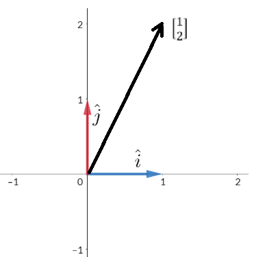
More conveniently, you may write a vector as [12] or simply v. Can you tell what the magnitude (or length or norm) of the above vector is?
Another way to represent a vector is by using basis vectors, i.e. ^ and ^, where ^=[10] and ^=[01]. Hence the vector [12] can be written as v=1^+2^.
Make sure you know how to add, subtract vectors, and also multiply/scale vectors by some scalar.
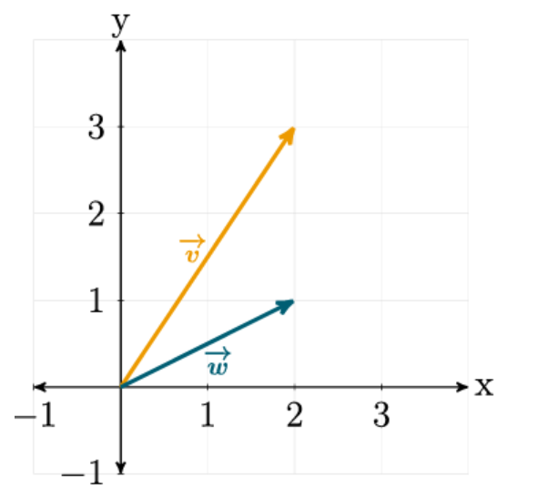
Try these ^^
(1) Express the above two vectors as column vectors and in ^,^ notation.
(2) Find also:
(a) v+w (b) v−w
(c) v+2w (d) v−2w
(3) Consider the following vectors:
u=⎣⎡−123⎦⎤,v=⎣⎡−123⎦⎤,w=⎣⎡45−2⎦⎤
Find:
(a) u+v (b) −u+2v−w (c) u⋅v (i.e. the dot product) (d) uTv (e) Which of the above vectors are orthogonal? (f) Express each of the vectors in ^,^,k^ notation.
We have already introduced the basis vectors ^ and ^, which we can put into a matrix. That is, the ^ and ^ vectors placed side-by-side in a 2×2 matrix:
This can easily be done by pre-multiplying the vector by the transformation matrix, as follows:
[01−10][12]=[−21]
Basically, a matrix can be viewed as a way to transform/change a vector!
Matrix addition and subtraction: If A=(aij) and B=(bij) are two m×n matrices of same dimension, then A+B is defined as (aij+bij). That is, we add element by element the two matrices. Clearly A+B=B+A. The rule applies to matrix subtraction.
Transpose of a matrix: If A is an m×n matrix, then A′ is the n×m matrix whose rows are the columns of A. So A′=(aji). For example:
Matrix Multiplication: The Column-Wise (Basis Vector) Method
Instead of dot products, we can view AB as taking the columns of A (the transformed ^ and ^) and scaling them by the components in each column of B.
From the sam eexample above, let the columns of A be:
a1=[13],a2=[2−4]
Finding Column 1 of the Result:
We use the first column of B[5−6] as scalars:
5[13]+(−6)[2−4]=[515]+[−1224]=[−739]
Finding Column 2 of the Result:
We use the second column of B[07] as scalars:
0[13]+7[2−4]=[00]+[14−28]=[14−28]
Final Result:
AB=[−73914−28]
as before!
Try these ^^
(1) For the following matrices:
A=[132−4],B=[5−607],
C=[12−364−5],D=[347−8−19].
Find:
(a) 5A−2B (b) 2A+3B (c) 2C−3D (d) AB and (AB)C (e) BC and A(BC)[Note that (AB)C=A(BC)] (f) A2 and A3 (g) AD and BD (h) CTD[Note that we cannot get CD. Why?] (i) A′ (j) B′ (k) A′B′ (l) (AB)′[Note that A′B′=(AB)′]
Diagonal matrix: A square n×n matrix A is diagonal if all entries off the ‘main diagonal’ are zero, i.e.
Symmetric matrix: A square matrix A is symmetric if A=A′. The identity matrix and the square null matrix are symmetric.
Idempotent matrix: A square matrix is said to be idempotent if An=⋯=A2=A. Below is an example (try squaring the matrix and see what you get).
[1000]
Singular Matrix: A matrix that is linearly dependent (in the columns or rows) is singular and has determinant of zero. Note that any two (or three) vectors x and y (and z) are said to be linearly dependent iff one can be written as a scalar multiple of the other. Two vectors x=0 and y=0 are said to be linearly independent iff the ONLY solution to ax+by=0 is a=0 AND b=0. And x and y are said to be orthogonal.
One of the uses of linear algebra in economics is to represent and then solve systems of equations. For instance, consider the system of two equations:
Matrix row operations, also known as elementary row operations, are three basic actions performed on a matrix: swapping two rows, multiplying a row by a non-zero constant, and adding a multiple of one row to another row.
Interchanging two rows (Row Swapping): You can swap the positions of any two rows in a matrix. As we will see later, this operation is useful for changing the order of equations in a system without altering the solution.
Multiplying a row by a non-zero constant (Scalar Multiplication): You can multiply every element in a specific row by any non-zero number. This is equivalent to multiplying both sides of an equation by a constant.
Adding a multiple of one row to another row (Row Addition): You can multiply one row by a constant and then add the result to another row. The original row and the row being multiplied remain unchanged. This operation is often the most powerful for simplifying systems, as it corresponds to adding a modified version of one equation to another.
Try these ^^
For the following matrices:
A=⎣⎡200030005⎦⎤,B=⎣⎡70000000−4⎦⎤,
C=⎣⎡200130205⎦⎤,D=⎣⎡7−2300100−4⎦⎤.
Find:
(a) Is the matrix A in REF or RREF? What are its pivots? (b) How about matrix B and C? Explain. (c) Change all matrices A to D to RREF (if they aren’t in RREF yet) and determine their rank.
We can solve system of equation by row operations.
To solve for x1 and x2, we can use an augmented matrix and perform elementary row operations—swapping rows, scalar multiplication, and row addition—to reach Reduced Row Echelon Form (RREF).
1. Set up the augmented matrix:
[2−111∣∣52]
2. Create a leading one in Row 1:
We can swap R1 and R2:
[−1211∣∣25]
Then multiply R1 by -1 to get a leading one (R1←−1⋅R1):
[12−11∣∣−25]
3. Create a zero below the leading one:
Add -2 times R1 to R2 (R2←R2−2R1):
[10−13∣∣−29]
4. Create a leading one in Row 2:
Multiply R2 by 1/3 (R2←31R2):
[10−11∣∣−23]
5. Create a zero above the leading one (RREF):
To reach reduced row echelon form, every column with a leading one must have zeros elsewhere. Add R2 to R1 (R1←R1+R2):
[1001∣∣13]
Basically, a matrix can be viewed as a way to transform or change a vector to solve these systems!
Final Result
The system provides the unique solution:
x1=1,x2=3
Basically, a matrix can be viewed as a way to transform or change a vector to solve these systems!
Note: We need not reach RREF, and could stop at Step 4 (or even Step 3). At Step 4, the last row tells us that x2=3. We can then use back-substitution into the first row (x1−x2=−2). HEnce x1−3=−2⟹x1=1.
This confirms the same result without performing the final row addition.
The determinant is a scalar value uniquely associated with a square non-singular matrix, and is usually denoted as ∣A∣. The question of whether or not a matrix is nonsingular and therefore invertible is linked to the value of its determinant.
We can write a generic 2×2 matrix as:
A=[a11a21a12a22]
and its determinant is defined as:
∣A∣=a11a22−a12a21
For a 3×3 matrix, say:
A=⎣⎡adgbehcfi⎦⎤
its determinant is:
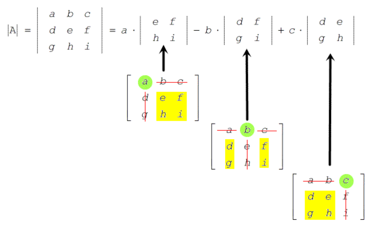
∣A∣=a(ei−fh)−b(di−fg)+c(dh−ef)
Note the sign in front of b is begative, because we imppose (multiply by) the sign matrix ⎣⎡+−+−+−+−+⎦⎤.
Visually:
The ‘yellow’ bits called minors are ‘smaller’ determinants, now 2 by 2 and easier to handle. Note that the elements of the minor come from remaining elements after deleting the rows and columns of the corresponding elements in the selected row (or column).
Let’s take a numerical example.
To find the determinant of matrix A using Cofactor Expansion along the first row (technically we could pick any row to work with) involves multiplying each element of the first row by its corresponding 2×2 minor, following the sign pattern: (+,−,+) for the first row.
Given:
A=⎣⎡213−3−1112−1⎦⎤
The formula for expansion along the first row is:
det(A)=a(M11)−b(M12)+c(M13)
1. First Element (a=2):
+2⋅∣∣−112−1∣∣=2⋅[(−1)(−1)−(2)(1)]=2(1−2)=−2
2. Second Element (b=−3):
Note the negative sign from the checkerboard pattern:
Property 2: Interchanging any two rows or columns will affect the sign of the determinant, but not its absolute value.
Property 3: Multiplying a single row or column by a scalar will cause the value of the determinant to be multiplied by the scalar.
Property 4: Addition or subtraction of a nonzero multiple of any row or column to or from another row or column does not change the value of the determinant.
Property 5: The determinant of a triangular matrix is equal to the product of the elements along the principal diagonal.
Property 6: If any of the rows or columns equal zero, the determinant is also zero.
Property 7: If two rows or columns are identical or proportional, i.e. linearly dependent, then the determinant is zero.
Note: Properties 2,3 and 4 are standard row operations already discussed above.
Where does the 10 in the matrix after the = sign come from? It is the determinant of A.
Then, (pre-)multiplying both sides of the equation by 101 gives:
101[4−321][13−24]=I
The matrix 101[4−321] is in fact the inverse of A.
Hence we have the relationship A−1A=I. In fact, A−1A=AA−1=I.
Finding the Inverse of a Matrix by Row Operations
We can find the inverse of a matrix using row operations or Gauss-Jordan Elimination method. The objective is to transform the matrix A into the Identity matrix I. By applying the same sequence of elementary row operations to an Identity matrix simultaneously, that Identity matrix transforms into A−1.
Given the matrix A from the example above
A=[13−24]
We set up an augmented matrix[A∣I] by placing the 2×2 Identity matrix to the right of A:
[A∣I]=[13−24∣∣1001]
Step-by-Step Row Operations
1. Create a zero below the first leading one:
Subtract 3 times the first row from the second row (R2←R2−3R1):
[10−210∣∣1−301]
2. Create a leading one in the second row:
Multiply the second row by 1/10 (R2←101R2):
[10−21∣∣1−3/1001/10]
3. Create a zero above the second leading one:
To reach Reduced Row Echelon Form (RREF), we add 2 times the second row to the first row (R1←R1+2R2):
[1001∣∣1+2(−3/10)−3/100+2(1/10)1/10]
Simplifying the arithmetic in the first row:
[1001∣∣4/10−3/102/101/10]
Final Result
The left side of the augmented matrix has been transformed into the Identity matrix. Therefore, the right side is now the inverse, A−1:
A−1=[0.4−0.30.20.1]
Verification
A matrix multiplied by its inverse must result in the Identity matrix:
Here are some properties of the inverse of a matrix worth knowing:
Property 1: For any nonsingular matrix A, (A−1)−1=A.
Property 2: The determinant of the inverse of a matrix is equal to the reciprocal of the determinant of the matrix. That is ∣A−1∣=∣A∣1.
Property 3: The inverse of matrix A is unique.
Property 4: For any nonsingular matrix A, the inverse of the transpose of a matrix is equal to the transpose of the inverse of the matrix. (A′)−1=(A−1)′.
Property 5: If A and B are nonsingular and of the same dimension, then AB is also nonsingular.
Property 6: The inverse of the product of two matrices is equal to the product of their inverses in reverse order. (AB)−1=B−1A−1.
Finding the Inverse of a Matrix (Standard Approach)