4 Correlation
By the end of this chapter, you should be able to:
- distinguish between univariate and bivariate data,
- use graphical tools to describe relationships between two variables,
- explain why means and standard deviations are insufficient for describing association,
- define and interpret the correlation coefficient,
- compute correlation using standard units,
- understand the limitations of correlation, especially with respect to causation.
4.1 Graphical representation
So far, we have focused on a single variable—what is known as univariate data—and examined their graphical and numerical summaries. We now turn to bivariate data, that is, data involving two variables.
As economists, we are often interested in understanding relationships between variables—for example, wages and education, CEO performance and salaries, economic growth and foreign aid, and many others. As with univariate data, both graphical and numerical summaries can be used.
The two most important graphical summaries for bivariate data are:
- Contingency tables, usually for categorical variables
- Scatter diagrams, usually for quantitative variables
A contingency table lists the frequency of each combination of values of two categorical variables. For example, a survey of 2,237 people recording gender and handedness might produce the following table.1
| Male | Female | |
|---|---|---|
| Right-handed | 934 | 1070 |
| Left-handed | 113 | 92 |
| Ambidextrous | 20 | 8 |
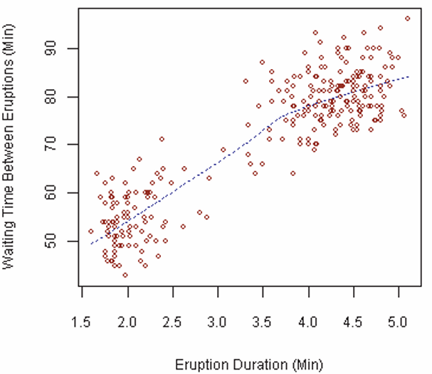
When dealing with cardinal (quantitative) data, the relationship between two variables is better visualized using a scatter diagram. The figure below shows the association between the duration of eruptions of Old Faithful and the waiting time between eruptions.
4.2 Correlation
Graphs are informative, but they also have limitations. For this reason, we need numerical summaries that describe the relationship between two variables.
In earlier chapters, we introduced the mean and standard deviation as the most important numerical summaries for univariate data. One might therefore ask: Why are these not sufficient for bivariate data?
Two datasets can have the same mean and standard deviation for each variable, yet exhibit very different relationships between those variables.
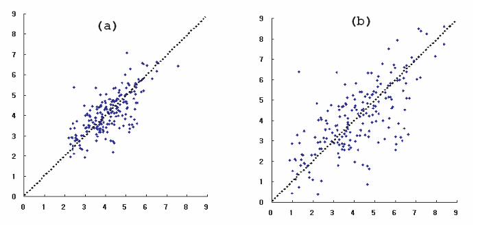
Consider a university that has offered two statistics sections, \(A\) and \(B\), over several years. For each student, midterm and final exam scores (out of 200) are recorded and plotted.
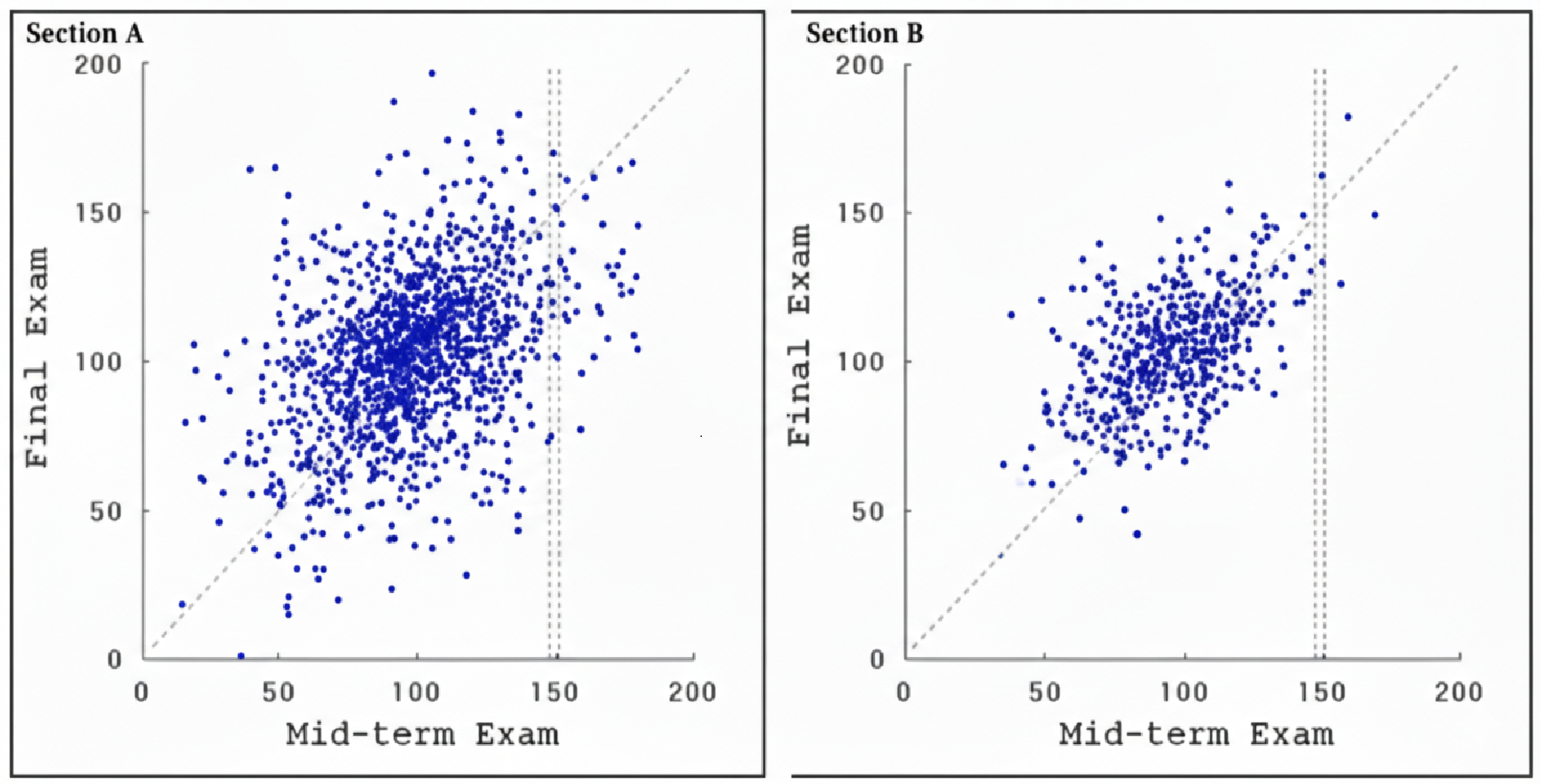
Points lying on the 45\(^\circ\) line represent students whose midterm and final scores are the same.
If there is a strong association, knowing one variable helps predict the other. If the association is weak, knowing one variable provides little predictive power.
For example, a student in section \(A\) who scored 150 on the midterm could plausibly score anywhere between 60 and 160 on the final. In section \(B\), a student with the same midterm score would likely score between 100 and 160. Midterm scores therefore provide better predictive information in section \(B\).
More strikingly, the means and standard deviations of both midterm and final scores are almost identical across the two sections. This means that we cannot distinguish the sections using only these summaries.
To capture how tightly points cluster around a line in a scatter diagram, we introduce the correlation coefficient, denoted by \(r\).
4.3 Correlation coefficient
The correlation coefficient is a pure number between \(-1\) and \(1\).
\[ -1 \leq Corr(X,Y) \leq 1 \]
Furthermore:
- \(r = 1\) or \(r = -1\) indicates perfect correlation
- A positive value of \(r\) indicates a positive relationship
- A negative value of \(r\) indicates a negative relationship
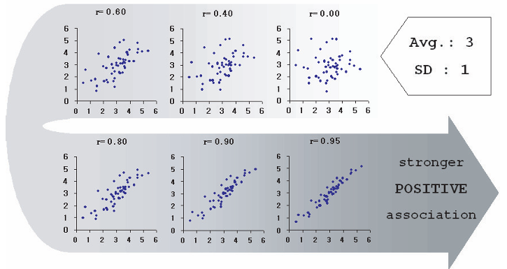
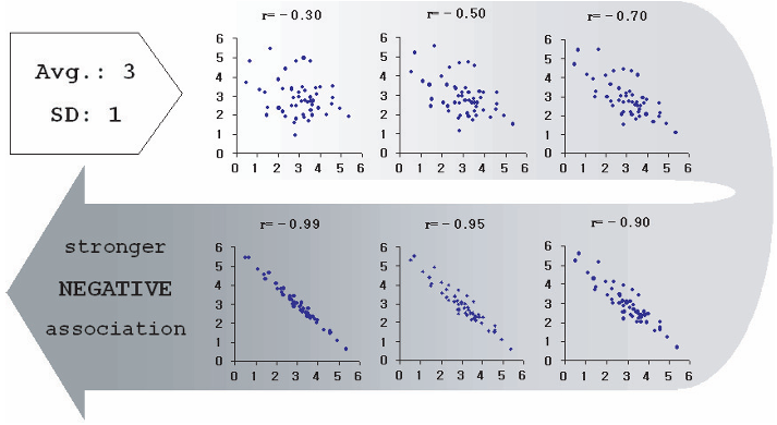
The figures below show two variables with the same mean (3) and standard deviation (1), but different correlations.
If either variable has a standard deviation equal to zero, then \(r = 0\). Correlation requires variation in both variables.
4.3.1 How correlation is computed
To compute the correlation coefficient:
- Convert each variable into standard units
- Multiply the standard units pairwise
- Take the average of these products
Standard units measure distance from the mean in terms of standard deviations.
For the list \(1, 3, 4, 5, 7\), the mean is 4 and the standard deviation is 2. The values in standard units are: \(-1.5,\; -0.5,\; 0,\; 0.5,\; 1.5\)
Standard units measure how far a value lies from the mean relative to the spread of the data.
Now consider the five points: \((1,5), (3,9), (4,7), (5,1), (7,13)\).
The mean of \(X\) is 4 with \(SD_X = 2\), and the mean of \(Y\) is 7 with \(SD_Y = 4\).
| X | Y | \(SU_X\) | \(SU_Y\) | Product |
|---|---|---|---|---|
| 1 | 5 | -1.5 | -0.5 | 0.75 |
| 3 | 9 | -0.5 | 0.5 | -0.25 |
| 4 | 7 | 0.0 | 0.0 | 0.0 |
| 5 | 1 | 0.5 | -1.5 | -0.75 |
| 7 | 13 | 1.5 | 1.5 | 2.25 |
The correlation coefficient is the average of the last column, which equals \(r = 0.4\).
4.3.2 Why this method matters
This approach shows that correlation:
- has no units
- is unchanged by rescaling variables
- measures relative, not absolute, clustering
There are many other ways to compute the correlation coefficient, but we will stick to the above method as it reveals best how the correlation coefficient works.
In many textbooks, the formula for correlation is written as:2
\[ Corr(X,Y) = \frac{\sum_{i=1}^{n} (X_i - \overline{X})(Y_i - \overline{Y})}{\sqrt{\sum_{i=1}^{n} (X_i - \overline{X})^2} \sqrt{\sum_{i=1}^{n} (Y_i - \overline{Y})^2}} \]
Another definition commonly used is:
\[ Corr(X,Y) = \displaystyle \frac{\text{Covariance}(X,Y)}{SD_x SD_y} \]
Compute the correlation coefficient for each of the following datasets.
(a)
| \(X\) | 1 | 1 | 1 | 1 | 2 | 2 | 2 | 3 | 3 | 4 |
|---|---|---|---|---|---|---|---|---|---|---|
| \(Y\) | 5 | 3 | 5 | 7 | 3 | 3 | 1 | 1 | 1 | 1 |
(b)
| \(X\) | 1 | 1 | 1 | 1 | 2 | 2 | 2 | 3 | 3 | 4 |
|---|---|---|---|---|---|---|---|---|---|---|
| \(Y\) | 1 | 2 | 1 | 3 | 1 | 4 | 1 | 2 | 2 | 3 |
(c)
| \(X\) | 1 | 1 | 1 | 1 | 2 | 2 | 2 | 3 | 3 | 4 |
|---|---|---|---|---|---|---|---|---|---|---|
| \(Y\) | 2 | 2 | 2 | 2 | 4 | 4 | 4 | 6 | 6 | 8 |
Question.
What do you observe about the values of the correlation coefficients across the three cases?
Note that the correlation coefficient is a pure number without any units, which is noted by the conversion to standard units.
Moreover, the correlation coefficient is *not** affected by any of the three changes: - 1) interchanging the two variables, - 2) adding the same number to all the values of one variable, and - 3) multiplying all the values of one variable by the same positive number.
This basically means that changing the scale of any of the variables leaves the correlation coefficient unchanged.
Be warned, looks can be deceiving. A quick glance at the above scatter plots would easily convince someone that the points in (a) is more tightly clustered, and thus having a correlation coefficient closer to 1, than (b). This cannot be further than the truth, because in fact = 0.7 for both diagrams. (b) is simply a magnification of (a). What is important to realize is that calculating involves converting variables to standard units (deviation from average divided by SD) and therefore it measures clustering not in absolute terms, but in relative terms (more specifically, relative to their standard deviations). That is, although plot (a) may appear more tightly clustered than plot (b), both have \(r = 0.7\). Plot (b) is simply a magnified version of plot (a). Correlation measures clustering relative to standard deviation, not in absolute terms.
The correlation coefficient captures linear relationships only. Nonlinear relationships may have low correlation even when variables are strongly related.
4.4 Association is not causation
The last piece of warning when using correlation coefficients is to realize that what we have is a representation of association, that is how the variables move relative to each other. The correlation coefficient does not establish causation. This is best left to economic theory, which is called upon to interpret and explain the data.
Correlation measures association, not causation.
A positive or negative correlation does not explain why variables move together. Establishing causation requires economic theory and careful empirical reasoning.
For example, education is often thought to cause higher wages because more educated individuals tend to earn more. However, a third factor—such as individual determination or motivation—may influence both education and wages.
Such a factor is known as a confounding variable, and its presence can invalidate causal interpretations based solely on correlation.
Correlation is a powerful descriptive tool, but causal claims require much more than a high value of \(r\).
Correlation provides a numerical summary of the strength and direction of linear association between two variables.
Scatter diagrams help visualize relationships, while the correlation coefficient measures how tightly points cluster around a straight line. However, correlation alone cannot establish causation, and careful reasoning is required to interpret empirical relationships correctly.
4.5 Exercises
4.5.1 Conceptual questions
Explain the difference between univariate and bivariate data.
Why are scatter diagrams useful for studying relationships between quantitative variables?
Explain why two datasets can have identical means and standard deviations but very different correlations.
4.5.2 Understanding correlation
What does the sign of the correlation coefficient indicate?
What does the magnitude of the correlation coefficient tell us?
Why must both variables exhibit variation for correlation to be meaningful?
A high correlation does not imply a causal relationship.
4.5.3 Computation and interpretation
Explain how converting variables to standard units removes units from the correlation coefficient.
Why is correlation unaffected by changes in scale or units?
Give an example of a nonlinear relationship that might have low correlation.
4.5.4 Optional challenge
- Find two real-world variables that are correlated.
Discuss whether the relationship is likely causal, and identify possible confounding variables.