5 The Normal Distribution
By the end of this chapter, you should be able to:
- explain why the normal distribution is central in statistics,
- state the probability density function of the normal distribution,
- interpret the mean \(\mu\) and variance \(\sigma^2\),
- apply the empirical (68–95–99.7) rule,
- standardize a normal random variable using \(z\)-scores,
- use the standard normal table to compute probabilities.
The Gaussian (normal) distribution is perhaps the most important continuous probability distribution in statistics.
Its importance stems largely from the Central Limit Theorem, which states that the sum (or average) of a large number of independent random variables will be approximately normally distributed — regardless of their individual distributions.
Any random variable that can be regarded as the sum of many small, independent contributions is therefore likely to follow an approximately normal distribution.
We return to this powerful result in Chapter 11.
5.1 The normal probability density function
A continuous random variable is said to be normally distributed with mean \(\mu\) and variance \(\sigma^2\) if its probability density function is
\[ f(x) = \frac{1}{\sigma \sqrt{2\pi}} e^{-\frac{1}{2}\left(\frac{x-\mu}{\sigma}\right)^2}. \]
The normal distribution is completely determined by two parameters:
- the mean \(\mu\)
- the variance \(\sigma^2\)
We write:
\[ X \sim N(\mu, \sigma^2). \]
- The distribution is symmetric about its mean.
- It extends from \(-\infty\) to \(+\infty\).
- The total area under the curve equals 1.
- Mean = median = mode.
Although the formula looks intimidating, in practice we rarely manipulate it directly. Instead, we standardize and use tables (or software).
5.2 The bell-shaped curve
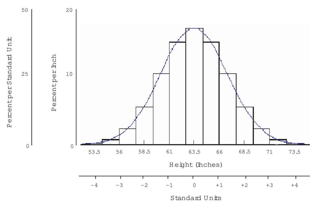
The empirical rule (also called the 68–95–99.7 rule) states:
- About 68% of observations lie within \(\pm 1\) standard deviation.
- About 95% lie within \(\pm 2\) standard deviations.
- About 99.7% lie within \(\pm 3\) standard deviations.
This rule provides quick approximations without using tables.
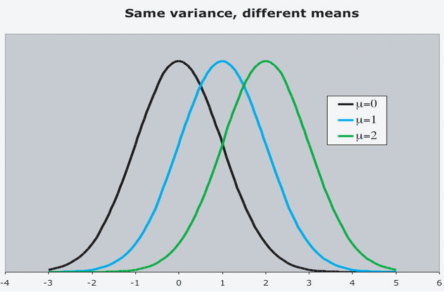
5.3 The role of mean and variance
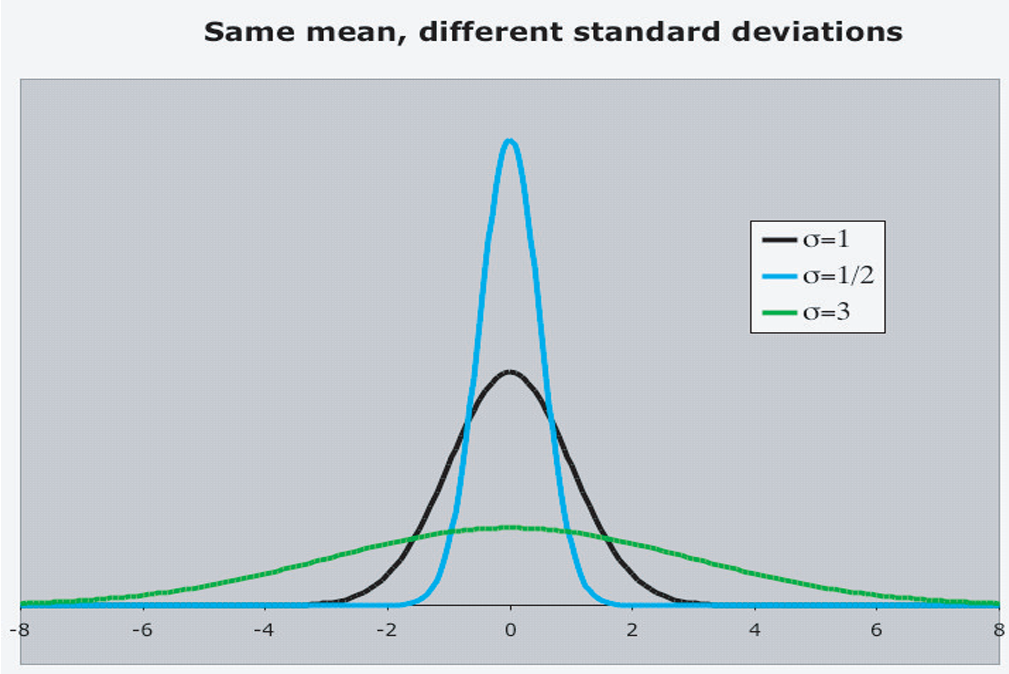
The normal distribution forms a family of curves.
- Changing \(\mu\) shifts the curve left or right.
- Changing \(\sigma\) stretches or compresses the curve.
5.4 Standardization and the standard normal distribution
To make probability calculations manageable, we standardize values.
The standardized value (or z-score) is:
\[ z = \frac{X - \mu}{\sigma}. \]
After standardization,
\[ z \sim N(0,1). \]
It has mean 0 and standard deviation 1.
Standardization allows us to use a single universal table.
5.5 Using the standard normal table
You can acccess the standard normal table from LINK
Suppose we want the area between the mean and \(z = 1.20\).
From the table:
\[ Pr(0 \le z \le 1.20) = 0.3849. \]
Instead of solving
\[ Pr(0 \le z \le 1.20) = \int_0^{1.20} \frac{1}{\sqrt{2\pi}} e^{-z^2/2} dz, \]
we simply look up the value.
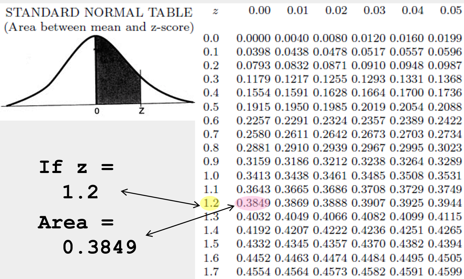
- Locate the \(z\) value in the first column.
- Read the corresponding area from the table.
Hence, \(Pr(0 \le z \le 1.20) = 38.49\%\).
5.5.1 Another Example:
For \(z = 1.35\).
- Find 1.3 in the first column.
- Move across to 0.05.
- The table value is 0.4115.
Hence, \(Pr(0 \le z \le 1.38) = 41.15 \%\).
5.6 Areas between two z-scores
To find:
\[ Pr(z_1 \le z \le z_2), \]
- Look up both areas from the mean.
- Add or subtract appropriately.
5.6.1 Example
To find:
\[ Pr(-1 \le z \le 2), \]
From the standard normal table, \(Pr(0 \le z \le 2) = 0.4772\), and \(Pr(0 \le z \le 1) = 0.3413 = Pr(-1 \le z \le 0)\), due to symmetry.
Hence, \(Pr(-1 \le z \le 2) = 0.4772 + 0.3413 = 0.8185\).
The table is make life even easier.
It allows us easily to look up the probabilities between the mean and some \(z\)-score.
But, even more, it allows to look up a \(z\)-score given some probability. This is the same as trying to solve:
\[ Pr(0 \leq z \leq z^*) = 0.45 = \int_0^{z^*} \frac{1}{\sigma \sqrt{2\pi}} e^{-\frac{1}{2}z^2} dx \]
which is quite intimidating!
5.6.2 Example
If we want to find the \(z\)-value corresponding to a probability of \(0.475\) between the mean and \(z\), we simply locate \(0.475\) (or the closest value) in the body of the standard normal table and then read off the corresponding \(z\)-score from the row and column headings. What do we get? \(1.96\)
5.7 Important benchmark
Approximately 95% of the area under the normal curve lies between
\[ -1.96 \text{ and } +1.96. \]
We often approximate this using \(\pm 2\).
5.8 Example: Heights
Suppose women’s heights have:
- mean \(= 160\) cm
- standard deviation \(= 5\) cm
We want:
\[ Pr(155 \le X \le 170). \]
Standardize:
\[ z = \frac{X - 160}{5}. \]
So:
- \(155 \rightarrow z = -1\)
- \(170 \rightarrow z = 2\)
Thus,
\[ Pr(-1 \le Z \le 2). \]
From the table:
\[ Pr(0 \le Z \le 1) = 0.3413, \]
\[ Pr(0 \le Z \le 2) = 0.4772. \]
Therefore,
\[ Pr(-1 \le Z \le 2) = 0.3413 + 0.4772 = 0.8185. \]
So approximately 82% of women fall in that height range.
The normal distribution plays a central role because:
- many natural phenomena are approximately normal,
- sums and averages tend toward normality,
- standardization allows universal probability tables.
The \(z\)-score is the key tool for translating real-world measurements into probabilities.
6 Problem Set
6.1 Conceptual questions
Why does the Central Limit Theorem make the normal distribution especially important?
Explain in words what the parameters \(\mu\) and \(\sigma^2\) represent.
Why must the total area under a probability density curve equal 1?
What does it mean for a distribution to be symmetric?
Why is standardization useful?
6.2 Empirical rule questions
If a normal distribution has mean 100 and SD 10, what proportion of observations lie between 80 and 120?
What proportion lies above 130?
Approximately what percentage lies below \(\mu - 3\sigma\)?
6.3 Standardization and table exercises
Suppose \(X \sim N(50, 9)\). Compute:
- \(Pr(X \le 53)\)
- \(Pr(47 \le X \le 56)\)
- \(Pr(X \le 53)\)
Suppose \(X \sim N(100, 16)\). Find \(z\) when \(X = 104\).
Find \(Pr(Z > 1.64)\).
Find \(z\) such that:
\[ Pr(0 \le Z \le z) = 0.45. \]
6.4 Applied problems
- Test scores are normally distributed with mean 70 and SD 8.
- What percentage score above 86?
- What percentage score between 62 and 78?
- IQ scores follow \(N(100, 15^2)\).
- What proportion have IQ above 130?
- What IQ corresponds to the top 5%?
- A factory produces rods with mean length 10 cm and SD 0.2 cm.
What percentage are longer than 10.4 cm?
- In Thailand, more than 1 million high school students took the university entrance exam in 1995. The average math score was 428 and the SD was 110.
- Estimate the 60th percentile of the math scores in 1995
- Among Bangkok schools, the average math score was 448 with SD
- About what percent of the Bangkok high-school students did better than the national average?
Replacement times for CD players are normally distributed with a mean of 7.1 years and a standard deviation of 1.4 years. If you want to provide a warranty so that only 2% of the CD players will be replaced before the warranty expires, what is the time length of the warranty
Men have a sitting heights that are normally distributed with a mean of 36.0 in. and a standard deviation of 1.4 in. The Honda Civic has a headroom of 39 in. What is the probability that a randomly selected man will not fit in the Civic? If you want to design a car so that 97% of men can fit it in, what should the headroom be?
6.5 Challenge question
- Show that standardizing a normal random variable produces a distribution with mean 0 and variance 1.