Warning: package 'ggplot2' was built under R version 4.5.3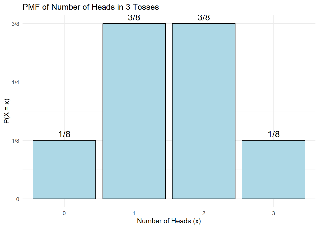
By the end of this chapter, you should be able to:
We begin by defining a random variable as a rule that assigns a number to each outcome of an experiment.
Instead of describing a single coin toss as \(\{\text{Heads}, \text{Tails}\}\), for example, we can “translate” outcomes into numbers such as 1 and 0. That numerical description is often more convenient — because once outcomes are numbers, we can compute averages, spreads, and relationships.
So a random variable is a bridge:
experiment \(\rightarrow\) outcomes \(\rightarrow\) numbers
A random variable is a function \(X\) that maps outcomes into real numbers:
\(X:\Omega \to \mathbb{R}\)
Here \(\Omega\) is the sample space (all possible outcomes).The experiment produces an outcome \(\omega \in \Omega\), and the random variable outputs the number \(X(\omega)\).
Once we have a random variable \(X\), we can ask:
How likely is each possible value of \(X\)?
A probability distribution answers this question by listing the possible values of \(X\) and the probability attached to each one.
Formally, if \(A\) is a set of real numbers, the probability that \(X\) falls in \(A\) is
\(P_X(A) = P(\{\omega \in \Omega : X(\omega)\in A\})\).
You do not need to memorize that expression. The idea is simple:
The probability that \(X\) lands in a set \(A\) equals the probability of all outcomes that map into \(A\).
A discrete random variable takes values that are separated and countable (often whole numbers like \(0,1,2,\dots\)).
A continuous random variable can take any value on an interval of the real line.
A helpful analogy:
\(P(X=x_i)=p_i,\quad p_i\ge 0,\quad \sum_i p_i = 1\)
\(P(a \le X \le b)=\int_a^b f(x)\,dx,\quad f(x)\ge 0,\quad \int_{-\infty}^{\infty} f(x)\,dx = 1\)
In earlier chapters, we used histograms, means, and standard deviations to summarize data.
In probability, we summarize random variables — and the key object is the probability distribution, which tells us how probabilities are allocated across possible outcomes.
Consider the experiment: toss a coin three times.
Let \(X\) be the random variable “number of heads in 3 tosses.”
The sample space has 8 equally likely outcomes. We can list outcomes and compute \(X\):
\[ \begin{array}{|c|c|} \hline \text{Outcome} & X = \text{No. of Heads} \\ \hline TTT & 0 \\ TTH & 1 \\ THT & 1 \\ THH & 2 \\ HTT & 1 \\ HHT & 2 \\ HTH & 2 \\ HHH & 3 \\ \hline \end{array} \] Outcomes of 3 tosses of a coin
From this we get the PMF (probability distribution) of \(X\):
\[ \begin{array}{|c|c|} \hline x & P(X=x) \\ \hline 0 & 1/8 = 0.125 \\ 1 & 3/8 = 0.375 \\ 2 & 3/8 = 0.375 \\ 3 & 1/8 = 0.125 \\ \hline \Sigma & 1.000 \\ \hline \end{array} \] Probability distribution of \(X\) = number of heads in 3 tosses
Warning: package 'ggplot2' was built under R version 4.5.3
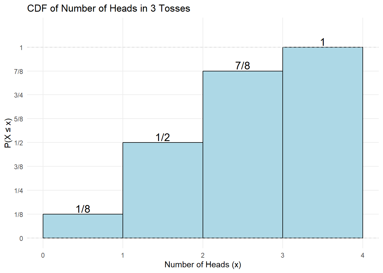
The CDF tells us \(P(X\le x)\) — the probability that the random variable is at most \(x\).
Apart from drawing the probability distribution or histograms, we have seen that numerical summaries such as the mean and variance are useful.
The mean is the long-run average value of a random variable, which is also referred to as its expected value, denoted \(E(X)\).1
\[ E(X) = \mu = \sum_{i=1}^{n} P(X_i) X_i \tag{7.1}\]
The variance which measures the spread or variation of the distribution is defined as:
\[ Var(X) = \sigma^2 = \sum_{i=1}^{n} P(X_i) (X_i- {\overline X})^2 \tag{7.2}\]
To get the standard deviation, simply calculate the square root of the variance.
It is easy to see that the formulas for expected value and variance are structurally identical—they are both weighted averages–to the “usual” formulas for mean and variance in previous chapters. The only difference is what weights are used.
Both \(E(X)\) and \(\mathrm{Var}(X)\) are weighted averages.
In samples, each observation often has equal weight \(1/n\).
In probability models, values are weighted by their probabilities.
Let’s apply the expected value and variance formulas with the example above which defines the random variable \(X\) as the number of heads in 3 tosses.
To compute the mean, use Equation 7.1, shown in the table below–summing the last column of the table gives \(\mu = 1.5\).
\[ \begin{array}{|c|c|c|} \hline X & P(X) & X \cdot P(X) \\ \hline 0 & 1/8 & 0 \\ 1 & 3/8 & 3/8 \\ 2 & 3/8 & 6/8 \\ 3 & 1/8 & 3/8 \\ \hline \textbf{Total} & \mathbf{1} & \mathbf{12/8 = 1.5} \\ \hline \end{array} \]
To get the variance, applying Equation 7.2, as shown in the the table below and summing the last column of the table gives \(\sigma^2 = 0.75\)
\[ \begin{array}{|c|c|c|c|} \hline X & P(X) & (X_i - \mu) & (X_i - \mu)^2 \cdot P(X) \\ \hline 0 & 0.125 & -1.5 & 0.28125 \\ 1 & 0.375 & -0.5 & 0.09375 \\ 2 & 0.375 & 0.5 & 0.09375 \\ 3 & 0.125 & 1.5 & 0.28125 \\ \hline \mathbf{\Sigma} & \mathbf{1.000} & & \sigma^2 = \mathbf{0.75} \\ \hline \end{array} \]
Careful, we have the variance \(=0.75\), hence the standard deviation \(\sigma = \sqrt{0.75}\) which is about \(0.8667\).
Let us introduce some basic rules of expected value and variance. Firstly, for expected value, we have:
Rule E1 \[E(k)=k\] Rule E2 \[E(X+k)=E(X)+k\]
Rule E3 \[E(kX)=kE(X)\]
Rule E1 states that the expected value (or average) of a constant is that constant. Rule E2 states that the expected value of a random variable to which a constant has been added is equal to the expected value of the random variable plus the constant. Rule E3 states that the expected value of a random variable multiplied by a constant is equal to the constant times the expected value of the random variable.
Secondly, the rules of variance are:
Rule V1 \[Var(k)=0\]
Rule V2 \[Var(X+k)=Var(X)\]
Rule V3 \[Var(kX)=k^2 Var(X)\]
Rule V1 states that the variance of a constant is zero (i.e., there is no spread). Rule V2 states that the variance of a random variable to which a constant has been added is simply equal to the variance of the random variable. Lastly, Rule V3 states that the variance of a random variable multiplied by a constant is equal to the constant squared times the variance of the random variable.2
Let’s illustrate how these rules apply to a real-world scenario.
The Data: For a food store, monthly sales have a mean (\(\mu\)) of Baht 25,000 and a standard deviation (\(\sigma\)) of Baht 4,000. Profits are defined as 30% of sales minus fixed costs of Baht 6,000.
The Goal: Find the mean and standard deviation of the monthly profit.
1. Define the Equation: \[Profit = 0.30(Sales) - 6,000\]
2. Calculate the Expected Value (Mean):
\[ \begin{aligned} V(\text{Profit}) &= V[0.30(\text{Sales}) - 6,000] \\ &= V[0.30(\text{Sales})] && \text{(Rules V2 \& V1)} \\ &= (0.30)^2 V(\text{Sales}) && \text{(Rule V3)} \\ &= 0.09 \cdot (4,000)^2 \\ &= 0.09 \cdot 16,000,000 \\ &= 1,440,000 \end{aligned} \]
3. Calculate the Variance and Standard Deviation: First, we find the variance (\(V\)). Remember that \(V(Sales) = \sigma^2 = 4,000^2\). \[ \begin{aligned} V(\text{Profit}) &= V[0.30(\text{Sales}) - 6,000] \\ &= V[0.30(\text{Sales})] && \text{(Rules V2 \& V1)} \\ &= (0.30)^2 V(\text{Sales}) && \text{(Rule V3)} \\ &= 0.09 \cdot (4,000)^2 \\ &= 0.09 \cdot 16,000,000 \\ &= 1,440,000 \end{aligned} \]
Finally, the standard deviation is: \[\sigma_{\text{Profit}} = \sqrt{1,440,000} = \mathbf{1,200}\]
So far, we have focused on univariate distributions. We now extend these ideas to bivariate probability distributions, which arise from joint probabilities.
A joint probability distribution of two discrete random variables \(X\) and \(Y\) is a table or formula that lists the joint probabilities for all pairs of values \((x, y)\). It is denoted by \(P(X,Y)\) or, equivalently, \(P(X = x \text{ and } Y = y)\).
As we would expect, joint probabilities satisfy the following basic properties:
\(0 \le P(X,Y) \le 1\)
and
\(\sum_x \sum_y P(X,Y) = 1\).
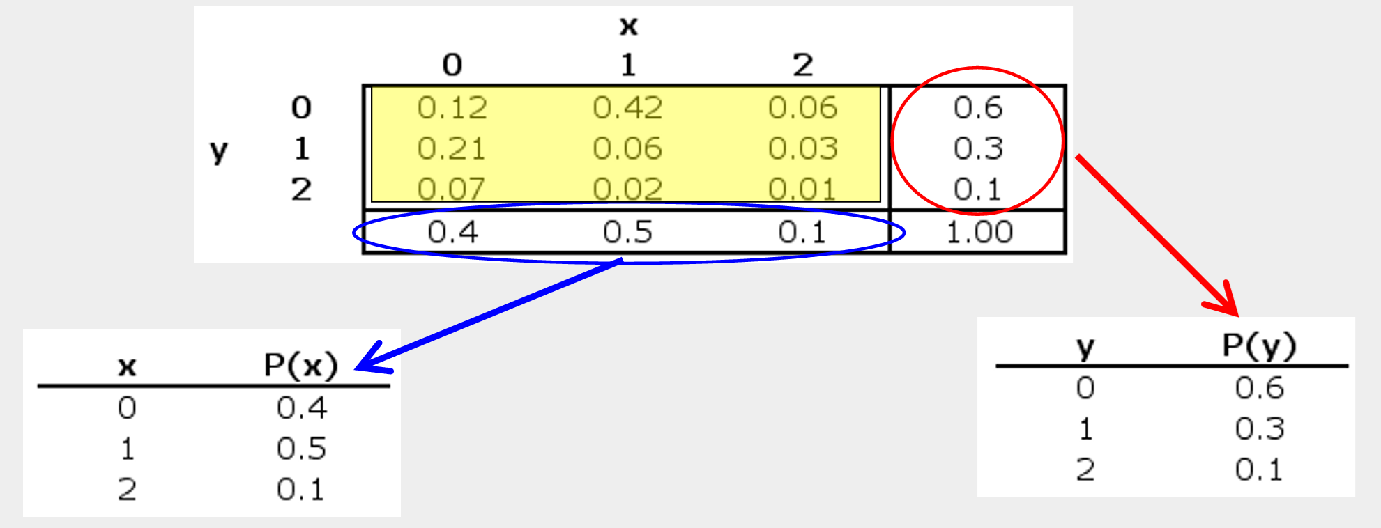
Let’s take an example. Xavier and Yvette are real estate agents; Let’s use X and Y to denote the number of houses each sells in a month, respectively. The following joint probabilities are based on past sales performance.
| x=0 | x=1 | x=2 | |
|---|---|---|---|
| Y=0 | 0.12 | 0.42 | 0.06 |
| Y=1 | 0.21 | 0.06 | 0.03 |
| Y=2 | 0.07 | 0.02 | 0.01 |
The marginal probabilities are obtained by summing the joint probabilities across rows or down the columns. They describe the probabilities of \(Y\) and \(X\) individually, ignoring the other variable.
Then using these marginal probabilities, we can compute the mean, and variance of each variable in a bivariate distribution by Equation 7.1 and Equation 7.2.
Check that you get \(E(X)=0.7\) and \(E(Y)=0.6\), respectively. How about the variances and standard deviations?3
The correlation coefficient is obtained by dividing the covariance by the product of the standard deviations:
\[ \text{Corr}(X,Y) = \dfrac{\text{Covariance}(X,Y)}{SD_X \, SD_Y} \]
Let’s try finding the correlation of Xavier and Yvette.
Starting from the covariance between two discrete random variables defined as
\[ Cov(X,Y) = P(X,Y) \sum_X \sum_Y (X - \overline{X})(Y - \overline{Y}) \tag{7.3}\]
or an alternative shorter formula is: \[ Cov(X, Y) = \sum_x \sum_y XY P(X, Y) - \overline{XY} \]
Try showing that the two equations are in fact the same.
Operationalizing Equation 7.3 gives
\[ \text{Covariance}(X,Y) = (0–.7)(0–.5)(.12) + (1–.7)(0-.5)(.42) + \dots + (2–.7)(2–.5)(.01) = –0.15 \]
Covariance measures whether \(X\) and \(Y\) tend to move together, while the correlation coefficient rescales covariance into a unit-free number:
\[ \mathrm{Corr}(X,Y)=\dfrac{\mathrm{Cov}(X,Y)}{\mathrm{SD}_X \mathrm{SD}_Y} \].
Correlation is always between \(-1\) and \(1\).
And finally, we get:
\[ \text{Corr} (X,Y) = \dfrac{-0.15}{0.64 \times 0.67} \approx -0.35 \]
A negative correlation meaning when Xavier does well, Yvette doesn’t (and vice-versa).
In this chapter, we introduced a random variable as a rule that assigns numbers to the outcomes of a random experiment, allowing us to analyze uncertainty mathematically.
A discrete probability distribution describes how probabilities are assigned to distinct values through a probability mass function (PMF). These probabilities must be nonnegative and sum to one.
We defined the expected value and variance as probability-weighted summaries of the distribution. The expected value represents the long-run average, while the variance measures dispersion around the mean.
Extending these ideas to two variables, we studied joint distributions, from which marginal distributions can be derived. Finally, we introduced covariance and correlation to measure the direction and strength of linear association between discrete random variables.
A discrete random variable \(X\) takes values \(x_1, x_2, \dots, x_k\) with probabilities \(P(X=x_i)\).
The random variable \(X\) has the following distribution:
| \(X\) | 0 | 1 | 2 | 3 |
|---|---|---|---|---|
| \(P(X)\) | 0.4 | 0.3 | 0.2 | 0.1 |
Let \(Y = 3X + 2\).
The joint probability distribution of \(X\) and \(Y\) is:
| \(Y=-1\) | \(Y=0\) | \(Y=1\) | |
|---|---|---|---|
| \(X=0\) | 0.1 | 0.1 | 0.1 |
| \(X=2\) | 0.1 | 0.2 | 0.1 |
| \(X=4\) | 0.1 | 0.1 | 0.1 |
Using the table in Question 5:
Let \(X\) be the number of heads when a fair coin is tossed three times.
Assume that the probability of a boy equals the probability of a girl and that births are independent.
The expected value is sometimes referred to as the population average; We will see later another definition of the expected value in later chpaters, as the “average” over infinite samples.↩︎
It is instructive to compare the expected value and variance rules with the summation rules.↩︎
These are sometimes referred to as moments–the mean and variance are the first moments and second central moments, respectively.
\[ \begin{array}{|c|c|c|c|} \hline \text{Order} & \text{Raw Moment} & \text{Central Moment} & \text{Common Name} \\ \hline \text{1st} & \mu_1' = E[X] & \mu_1 = E[X - E[X]] = 0 & \text{Mean} \\ \hline \text{2nd} & \mu_2' = E[X^2] & \mu_2 = E[(X - \mu)^2] & \text{Variance} \\ \hline \text{3rd} & \mu_3' & \mu_3 = E[(X - \mu)^3] & \text{Skewness} \\ \hline \text{4th} & \mu_4' & \mu_4 = E[(X - \mu)^4] & \text{Kurtosis} \\ \hline \end{array} \]↩︎