8 Binomial and Poisson Distributions
By the end of this chapter, you should be able to:
- apply basic counting principles (permutations and combinations),
- derive and use the binomial probability formula,
- compute probabilities for “exactly \(x\) successes” problems,
- understand when the normal distribution approximates the binomial,
- define and apply the Poisson distribution,
- recognize when binomial and Poisson models are appropriate.
- briefly introduce the geometric and negative binomial distribution.
- briefly mention the hypergeometric distribution.
8.1 Counting principles
Before introducing the binomial formula, we need a short detour into counting.
Probability often reduces to a simple question:
How many possible outcomes are there?
8.1.1 The multiplication rule of counting
If one task can be performed in \(m\) ways and a second task in \(n\) ways, then the two tasks together can be performed in \(m \times n\) ways.
Example:
A restaurant offers 3 starters and 4 main courses.
The number of possible meals is:
\[ 3 \times 4 = 12. \]
This simple idea lies behind much of probability theory.
8.1.2 Permutations
A permutation counts the number of ways to arrange objects when order matters.
The number of ways to arrange \(n\) distinct objects is:
\[ n! = n(n-1)(n-2)\dots 1. \]
If we choose \(k\) objects out of \(n\) and order matters, the number of permutations is:
\[ P(n,k) = \frac{n!}{(n-k)!}. \]
8.1.3 Combinations
A combination counts the number of ways to choose objects when order does not matter.
The number of combinations of \(k\) objects from \(n\) is:
\[ \binom{n}{k} = \frac{n!}{k!(n-k)!}. \]
This expression is called the binomial coefficient.
It plays a central role in the binomial distribution.
8.2 The Binomial Distribution
We often encounter problems of the form:
- A coin is tossed 4 times. What is the probability of exactly 1 head?
- A die is rolled 10 times. What is the probability of exactly 3 sixes?
- A box contains 1 red and 9 green marbles. Five draws are made with replacement. What is the probability of exactly 2 red marbles?
These are examples of binomial experiments.
8.2.1 Conditions for a binomial model
A binomial model applies when:
- The number of trials \(n\) is fixed.
- Each trial has two possible outcomes (success/failure).
- The probability of success \(p\) is constant.
- The trials are independent.
8.2.2 Box Model Example
Let’s look more closely at the last example above. We might start with a box model:
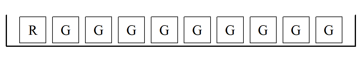
From the above, we draw 5 tickets at random with replacement. But we want exactly 2 R’s and 3 G’s (e.g., \(\fbox{R}, \fbox{R}, \fbox{G}, \fbox{G}, \fbox{G}\) or \(\fbox{G}, \fbox{R}, \fbox{G}, \fbox{G}, \fbox{R}\), etc.). The exact probability can be found using 3 simple steps:
1) Find all the possible ways: \[ \frac{5!}{2! \times 3!} = \frac{\text{total cases}}{\text{no. of successes} \times \text{no. of failures}} \]
2) Calculate the chance of each: \[ \frac{1}{10} \times \frac{1}{10} \times \frac{9}{10} \times \frac{9}{10} \times \frac{9}{10} = \left( \frac{1}{10}\right)^2 \left( \frac{9}{10}\right)^3 \]
3) Use the addition rule to add up the chances: \[ \frac{5!}{2! \times 3!} \times \left( \frac{1}{10}\right)^2 \left( \frac{9}{10}\right)^3 \approx 7\% \]
This can be interpreted as the chance of getting exactly 2 \(\fbox{R}\)’s.
Note that step 1 is actually the binomial coefficient, which gives us the total number of combinations of arranging 2 R’s and 3 G’s. In step 2, the chance of getting \(\fbox{R}, \fbox{R}, \fbox{G}, \fbox{G}, \fbox{G}\) is the same as getting \(\fbox{G}, \fbox{R}, \fbox{G}, \fbox{G}, \fbox{R}\), and so on. Lastly, step 3 involves the addition rules as all events are mutually exclusive (disjoint).
8.2.3 The Binomial Formula
If \(X\) counts the number of successes in \(n\) independent trials with success probability \(p\), then
\[ P(X = x) = \binom{n}{x} p^x (1-p)^{n-x}, \quad x = 0,1,\dots,n. \]
Where:
- \(n\) = number of trials
- \(x\) = number of successes
- \(p\) = probability of success
In short, we can write \(X \sim \text{Bin}(n, p)\).
8.2.4 Example
A neighbor has 3 children. What is the probability exactly 2 are boys?
Assuming \(p = 1/2\),
\[ P(X=2) = \binom{3}{2} \left(\frac{1}{2}\right)^2 \left(\frac{1}{2}\right)^1 = \frac{3}{8}. \]
This is exactly the same as the probability of 2 heads in 3 coin tosses.
Note that you can get all \(P(X=0), P(X=1), P(X=2), and P(X=3),\) using the binomial formula, i.e.e the entire distribution corresponding to the probability of no boys, one boy, … , all three boys for my neighbor with 3 children!
8.2.5 Mean and variance of the binomial
If \(X \sim \text{Bin}(n,p)\), then
\[ E(X) = np \]
\[ \text{Var}(X) = np(1-p) \]
These formulas are extremely useful.
Let \(X \sim \text{Bin}(n, p)\), where the probability mass function is:
\[P(X = x) = \binom{n}{x} p^x (1-p)^{n-x}\]
1. Derivation of the Mean or Expected Value
By definition, the expected value is:
\[E(X) = \sum_{x=0}^{n} X \cdot P(X=x) = \sum_{x=0}^{n} X \binom{n}{x} p^x (1-p)^{n-x}\]
Drop the \(X=0\) term, since the first term is \(0 \cdot P(X=0)\), we can start the sum at \(X=1\).
We can simplify the combination by the identity \(X \binom{n}{x} = n \binom{n-1}{x-1}\).
\[E(X) = \sum_{x=1}^{n} n \binom{n-1}{x-1} p^x (1-p)^{n-x}\]
Factor out \(np\). That is, pull a \(n\) and one \(p\) outside the summation.
\[E(X) = np \sum_{x=1}^{n} \binom{n-1}{x-1} p^{x-1} (1-p)^{n-x}\]
Let’s re-index the sum. Let \(k = x-1\). As \(x\) goes from \(1\) to \(n\), \(k\) goes from \(0\) to \(n-1\).
\[E(X) = np \sum_{k=0}^{n-1} \binom{n-1}{k} p^k (1-p)^{(n-1)-k}\]
Apply the Binomial Theorem. The entire summation is just the expansion of \((p + (1-p))^{n-1}\). Since \((p + 1 - p) = 1\), the sum is \(1^{n-1} = 1\).
\[E(X) = np \times 1 = np\]
Another way to see this, which is quicker, is to think of a Binomial random variable \(X\) as the sum of \(n\) independent Bernoulli trials (\(X_1, X_2, \dots, X_n\)), where each \(X_i\) is 1 for a success and 0 for a failure.
\[X = X_1 + X_2 + \dots + X_n\]
Hence, the mean of a single trial is \(E(X_i) = (1 \times p) + (0 \times (1-p)) = p\).
And using the linearity of expectation, the expected value of a sum is the sum of the expected values:
\[E(X) = E(X_1) + E(X_2) + \dots + E(X_n)\]
So,
\[ E(X) = p + p + \dots + p = np \]
2. Derivation of the Variance
To derive the variance of a binomial distribution, we typically use the formula:
\[ \text{Var}(X) = E(X^2) - [E(X)]^2 \]
Since we already know that \(E(X) = np\), we only need to find \(E(X^2)\).
A common “trick” in discrete math is to rewrite \(X^2\) as \(X(X-1) + X\). This allows us to use the same combination-reduction trick we used for the mean.
\[\text{Var}(X) = E(X(X-1)) + E(X) - [E(X)]^2\]
First, calculate \(E(X(X-1))\):
Using the PMF of the binomial distribution:
\[E[X(X-1)] = \sum_{X=0}^{n} X(X-1) \binom{n}{x} p^x (1-p)^{n-x}\]
Here again the terms for \(X=0\) and \(X=1\) are zero, so the sum starts at \(X=2\).
Let’s reduce the combination. Use the identity \(X(X-1) \binom{n}{x} = n(n-1) \binom{n-2}{x-2}\).
\[E[X(X-1)] = \sum_{x=2}^{n} n(n-1) \binom{n-2}{x-2} p^x (1-p)^{n-x}\]
And factor out constants, i.e. pull out \(n(n-1)\) and \(p^2\).
\[E[X(X-1)] = n(n-1)p^2 \sum_{x=2}^{n} \binom{n-2}{x-2} p^{x-2} (1-p)^{n-x}\]
Lastly sum to 1. Just like in the mean derivation, the remaining sum is the binomial expansion of \((p + (1-p))^{n-2}\), which equals \(1\).
\[E[X(X-1)] = n(n-1)p^2\]
Now substitute everything back into the variance formula:
\[\text{Var}(X) = E(X(X-1)) + E(X) - [E(X)]^2\]
\[\text{Var}(X) = n(n-1)p^2 + np - (np)^2\] Expand terms:
\[\text{Var}(X) = n^2p^2 - np^2 + np - n^2p^2\]
The \(n^2p^2\) terms cancel out, leaving
\[\text{Var}(X) = np - (np)^2 = np(1-p)\]
The intuitive shortcut, if you prefer, is to use the linearity of expectation approach again. The variance of a single Bernoulli trial (\(X_i\)) is \(p(1-p)\). Since the trials are independent, the variance of the sum is the sum of the variances:
\[\text{Var}(X_1 + \dots + X_n) = \text{Var}(X_1) + \dots + \text{Var}(X_n)\]
So,
\[\text{Var}(X) = p(1-p) + \dots + p(1-p) = np(1-p)\]
8.3 Normal approximation to the binomial distribution
When \(n\) is large, calculating binomial probabilities directly can be tedious.
Fortunately, the Central Limit Theorem tells us that the binomial distribution becomes approximately normal when \(n\) is large.
If
\[ X \sim \text{Bin}(n,p), \]
then for sufficiently large \(n\),
\[ X \approx N\big(np,\; np(1-p)\big). \]
That is:
- Mean \(= np\)
- Variance \(= np(1-p)\)
- Standard deviation \(= \sqrt{np(1-p)}\)
8.3.1 When is the approximation good?
A common rule of thumb is:
\[ np \ge 5 \quad \text{and} \quad n(1-p) \ge 5. \]
8.3.2 Continuity correction
Because the binomial distribution is discrete and the normal distribution is continuous, we use a continuity correction.
For example:
To approximate \(P(X \le 10)\), compute
\[ P(X \le 10.5) \]
using the normal distribution.
8.3.2.1 Example
Suppose \(X \sim \text{Bin}(100, 0.5)\).
Mean: \[ \mu = np = 50 \]
Standard deviation: \[ \sigma = \sqrt{100(0.5)(0.5)} = 5. \]
To approximate
\[ P(X \ge 60), \]
we compute
\[ P\left(Z \ge \frac{59.5 - 50}{5}\right). \]
The rest follows using the standard normal table.
8.3.2.2 Another Example
Suppose a fair coin is tossed \(100\) times.
Let \(X\) be the number of heads.
Then
\[ X \sim \text{Bin}(100, 0.5). \]
Step 1: Compute mean and standard deviation
\[ \mu = np = 100(0.5) = 50 \]
\[ \sigma = \sqrt{np(1-p)} = \sqrt{100(0.5)(0.5)} = 5. \]
1: Approximate \(P(X \ge 60)\)
Step 2: Apply continuity correction
Because the binomial is discrete, we approximate:
\[ P(X \ge 60) \approx P(X \ge 59.5). \]
Step 3: Convert to a \(z\)-score
\[ z = \frac{59.5 - 50}{5} = \frac{9.5}{5} = 1.9. \]
Step 4: Use the standard normal table
From the table:
\[ P(Z \le 1.9) = 0.9713. \]
Therefore,
\[ P(Z \ge 1.9) = 1 - 0.9713 = 0.0287. \]
Final Answer
\[ P(X \ge 60) \approx 0.0287. \]
So there is roughly a \(2.9\%\) chance of obtaining 60 or more heads.
2: Approximate \(P(45 \le X \le 55)\)
Step 2: Continuity correction
\[ P(45 \le X \le 55) \approx P(44.5 \le X \le 55.5). \]
Step 3: Convert to \(z\)-scores
Lower bound:
\[ z_1 = \frac{44.5 - 50}{5} = -1.1. \]
Upper bound:
\[ z_2 = \frac{55.5 - 50}{5} = 1.1. \]
Step 3: Look up table values
From the standard normal table:
\[ P(0 \le Z \le 1.1) = 0.3643. \]
By symmetry:
\[ P(-1.1 \le Z \le 1.1) = 2(0.3643) = 0.7286. \]
Final Answer
\[ P(45 \le X \le 55) \approx 0.7286. \]
So about \(73\%\) of the time, the number of heads will fall between 45 and 55.
8.4 The Poisson Distribution
The Poisson distribution models the number of events occurring in a fixed interval of time or space when events occur:
- independently,
- randomly,
- at a constant average rate.
Typical examples:
- Number of calls per hour,
- Number of defects per page,
- Number of accidents per month.
8.5 The Poisson Formula
If \(X\) follows a Poisson distribution with mean \(\mu\), then
\[ P(X = x) = \frac{e^{-\mu} \mu^x}{x!}, \quad x = 0,1,2,\dots \]
Where:
- \(\mu\) = average number of events,
- \(e \approx 2.71828\).
8.5.1 Mean and variance
For a Poisson distribution:
\[ E(X) = \mu \]
\[ \text{Var}(X) = \mu. \]
Thus, the mean and variance are equal.
8.5.2 Example
If typographical errors follow a Poisson distribution with mean \(\mu = 1.5\) per 100 pages, then
\[ P(X=0) = \frac{e^{-1.5} 1.5^0}{0!} = e^{-1.5} \approx 0.2231. \] which represents the probability of no errors in a 100 pages.
Here, again we can use the Poisson formula to find \(P(X=1), P(X=2), \dots\) corresponding to the probability of one error, two errors per 100 pages, and so on.
8.6 Binomial–Poisson connection
When:
- \(n\) is large,
- \(p\) is small,
- and \(\mu = np\) remains moderate,
the binomial distribution can be approximated by a Poisson distribution:
\[ \text{Bin}(n,p) \approx \text{Poisson}(\mu = np). \]
This is especially useful for modeling rare events.
8.7 The Geometric and Negative Binomial Distribution
8.8 The Hypergeometric Distribution
The binomial distribution models the number of successes in repeated independent trials with constant probability \(p\), while the Poisson distribution models rare events occurring over time or space with average rate \(\mu\). The binomial has mean \(np\) and variance \(np(1-p)\); the Poisson has mean and variance both equal to \(\mu\). For large samples, the binomial distribution can be approximated by the normal distribution using standardization with \(z\)-scores. Together, these models allow us to quantify uncertainty in repeated trials, rare events, and large-sample settings.
8.9 Exercises
8.9.1 Conceptual Understanding
What are the four conditions required for a binomial experiment?
Explain why independence of trials is crucial for the binomial formula.
When is the Poisson distribution more appropriate than the binomial?
Why does the normal approximation improve as \(n\) increases?
8.9.2 Binomial Calculations
A multiple-choice test has 20 questions with 4 possible answers each.
- If a student guesses randomly, what is the probability of exactly 8 correct answers?
- What are the mean and standard deviation?
- If a student guesses randomly, what is the probability of exactly 8 correct answers?
A manufacturing process produces defective items with probability \(p = 0.02\).
- In a batch of 50 items, what is the probability of exactly 1 defect?
- What is the probability of no defects?
- In a batch of 50 items, what is the probability of exactly 1 defect?
8.9.3 Normal Approximation
Suppose \(X \sim \text{Bin}(200, 0.4)\).
- Compute the mean and standard deviation.
- Approximate \(P(X \ge 90)\) using the normal approximation.
- Clearly show the continuity correction and \(z\)-steps.
- Compute the mean and standard deviation.
A factory produces lightbulbs with defect probability \(p = 0.1\).
In a shipment of 120 bulbs:
- Approximate the probability that between 8 and 18 bulbs are defective.
- Compare your answer to what you expect intuitively.
- Approximate the probability that between 8 and 18 bulbs are defective.
8.9.4 Poisson Applications
Customers arrive at a bank at an average rate of 3 per minute.
- What is the probability that exactly 5 customers arrive in one minute?
- What is the probability that no customers arrive in two minutes?
- What is the probability that exactly 5 customers arrive in one minute?
Calls arrive at a call center at a rate of 2 per hour.
- What is the probability of 6 or more calls in one hour?
- What is the probability of exactly 1 call in 30 minutes?
- What is the probability of 6 or more calls in one hour?
8.9.5 Synthesis
- Under what conditions can:
- The binomial be approximated by the normal?
- The binomial be approximated by the Poisson?
- Suppose \(n\) is very large and \(p\) is very small.
Explain intuitively why the Poisson distribution emerges from the binomial.