Chapter 1 — Why Time Series Matter
Many of the most important phenomena in economics, business, finance, and society evolve through time.
Inflation changes from month to month.
Stock prices fluctuate every second.
GDP rises and falls over business cycles.
Exchange rates respond continuously to news and expectations.
Understanding these dynamic patterns is one of the central goals of time series analysis.
This book introduces the core ideas of applied time series analysis using:
economic and financial data
visualization and intuition
forecasting applications
trading examples
Python and Gretl
The emphasis throughout is practical and data-driven.
Learning Objectives
By the end of this chapter, you should be able to:
explain what a time series is
distinguish time series data from cross-sectional data
explain why time matters in economics and finance
understand the importance of dependence and dynamics
identify trends, cycles, and noise
understand why forecasting is difficult
recognize major applications of time series analysis
1.1 The World Changes Through Time
Many variables are not static.
They evolve.
Examples include:
inflation
unemployment
stock prices
GDP
interest rates
exchange rates
commodity prices
electricity demand
cryptocurrency prices
Unlike purely cross-sectional analysis, time series analysis focuses on:
dynamics
persistence
trends
cycles
forecasting
uncertainty
1.2 What Is a Time Series?
A time series is a sequence of observations ordered through time.
Examples include:
| Variable | Frequency |
|---|---|
| monthly inflation | monthly |
| quarterly GDP | quarterly |
| daily stock prices | daily |
| hourly electricity demand | hourly |
| second-by-second Bitcoin prices | high frequency |
We often represent a time series as:
where:
denotes the value observed at time
is the final observation
1.3 Why Economists Care About Time
Economic systems are dynamic.
Governments, firms, and households continuously respond to changing conditions.
Economists therefore study variables such as:
inflation
unemployment
GDP growth
interest rates
exchange rates
through time.
Business Cycles
Economic activity tends to fluctuate.
Periods of expansion are often followed by slowdowns or recessions.
Understanding these cycles is one of the main goals of macroeconomics.
Inflation Dynamics
Inflation often displays persistence.
High inflation this month may increase the probability of high inflation next month.
Central banks therefore monitor inflation continuously.
Forecasting
Economic forecasting is crucial for:
monetary policy
fiscal planning
investment decisions
budgeting
risk management
1.4 Why Financial Markets Care About Time
Financial markets are highly dynamic systems.
Prices react continuously to:
news
expectations
policy changes
earnings announcements
geopolitical events
Even small changes can matter enormously.
Traders and Investors
Traders care about:
returns
volatility
trends
momentum
reversals
timing
Portfolio managers care about:
risk
diversification
correlations
forecasting volatility
Algorithmic Trading
Modern financial markets increasingly rely on automated systems.
Algorithms monitor time series data in real time to:
detect patterns
generate trading signals
manage risk
execute trades
1.5 Time Series vs Cross-Sectional Data
It is important to distinguish time series data from cross-sectional data.
Cross-Sectional Data
Cross-sectional data observe many units at a single point in time.
Example:
| Country | Inflation Rate |
|---|---|
| Thailand | 2.1 |
| Japan | 0.5 |
| Indonesia | 3.0 |
The focus is on differences across units.
Time Series Data
Time series data observe one variable repeatedly through time.
Example:
| Month | Inflation |
|---|---|
| January | 2.1 |
| February | 2.3 |
| March | 2.5 |
The focus is on dynamics through time.
1.6 Why Dependence Matters
In many time series, the past influences the future.
This idea is called dependence.
For example:
inflation today may depend on inflation yesterday
stock volatility today may depend on volatility yesterday
GDP growth this quarter may depend on previous quarters
This is fundamentally different from many standard statistical models that assume observations are independent.
Examples of Dependence
Inflation Persistence
Inflation often changes gradually rather than randomly jumping each month.
Volatility Clustering
Financial markets often display calm periods followed by turbulent periods.
Large movements tend to cluster together.
Momentum
Stocks that recently increased in price sometimes continue rising temporarily.
1.7 Trend, Cycles, and Noise
Many time series contain several components.
Trend
A trend represents long-run movement.
Examples include:
long-run GDP growth
long-run population growth
long-run technological progress
Cycles
Cycles are recurring fluctuations around the trend.
Examples include:
business cycles
seasonal shopping patterns
tourism cycles
Noise
Noise represents random fluctuations that are difficult to predict.
1.8 Forecasting and Decision Making
Forecasting plays a central role in economics and business.
| Forecast | Decision |
|---|---|
| inflation | interest rate policy |
| demand | inventory planning |
| exchange rates | hedging |
| volatility | portfolio risk |
| sales | staffing decisions |
Examples
Airlines forecast passenger demand.
Banks forecast interest rates.
Retailers forecast seasonal sales.
Governments forecast economic growth.
1.9 Why Forecasting Is Difficult
Forecasting is inherently uncertain.
Why?
Because economies and markets are affected by:
unexpected shocks
policy changes
crises
technological change
human behavior
Even strong statistical models cannot perfectly predict the future.
Financial Markets
Financial markets are especially difficult to forecast because prices rapidly incorporate information.
New information arrives continuously and unpredictably.
Structural Breaks
Relationships may change over time.
For example:
financial crises
pandemics
wars
regime changes
can alter economic dynamics dramatically.
1.10 Time Series in the Age of AI
The importance of time series analysis has increased dramatically in recent years.
Modern applications include:
algorithmic trading
recommendation systems
streaming data analysis
sensor monitoring
real-time forecasting
AI-driven prediction systems
Large amounts of sequential data are now generated continuously.
Examples include:
online recommendation systems
fraud detection
autonomous vehicles
smart factories
high-frequency trading systems
1.11 A First Look at Financial Data with Python
We now download and plot real financial data using Python.
# !pip install yfinance

import matplotlib.pyplot as plt
import yfinance as yf

# Download S&P 500 data
sp500 = yf.download("^GSPC", start="2018-01-01", auto_adjust=False)

# Inspect the columns to confirm
# print(data.columns)

# Plot the adjusted close price
sp500["Adj Close"].plot(figsize=(10,4))

plt.title("S&P 500 Adjusted Closing Price")
plt.xlabel("Date")
plt.ylabel("Index Level")

plt.savefig("figs/ch1/sp500.png", dpi=300, bbox_inches="tight")
plt.close()   # replace with plt.show()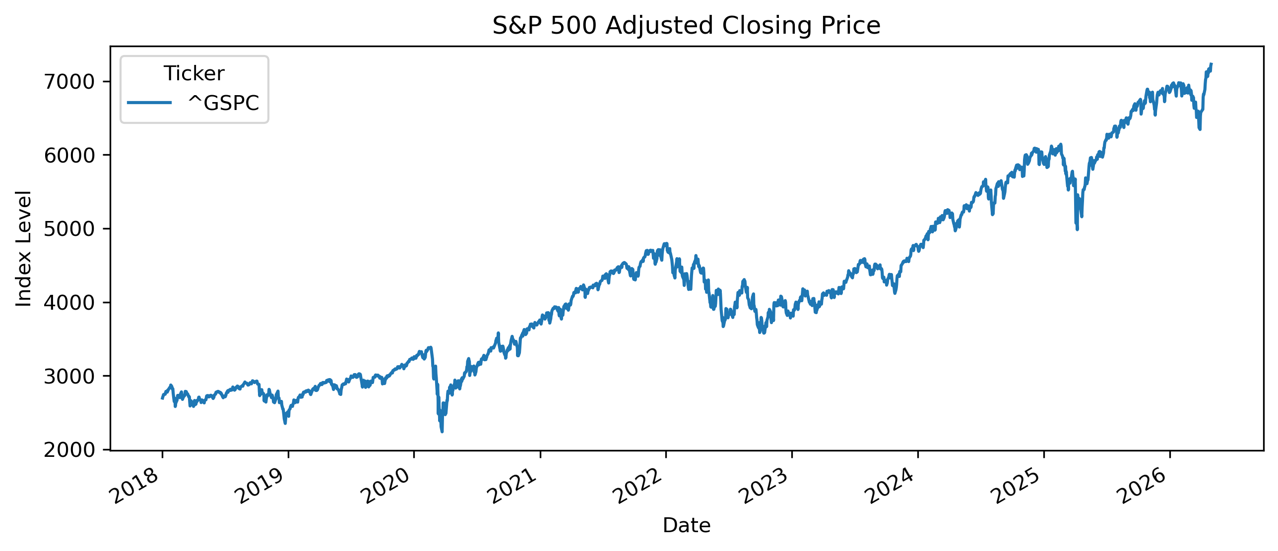
You can also try:
# Download Netflix data
data = yf.download("NFLX", start="2020-01-01", end="2026-04-31", auto_adjust=False)1.12 Example: Exchange Rates
Exchange rates are another important example of time series data.
# import yfinance as yf
# import matplotlib.pyplot as plt

thb = yf.download("THB=X", start="2020-01-01", auto_adjust=False)

thb["Adj Close"].plot(figsize=(10,4))

plt.title("Thai Baht per U.S. Dollar")
plt.xlabel("Date")
plt.ylabel("Exchange Rate")

plt.savefig("figs/ch1/xr.png", dpi=300, bbox_inches="tight")
plt.close()   # replace with plt.show()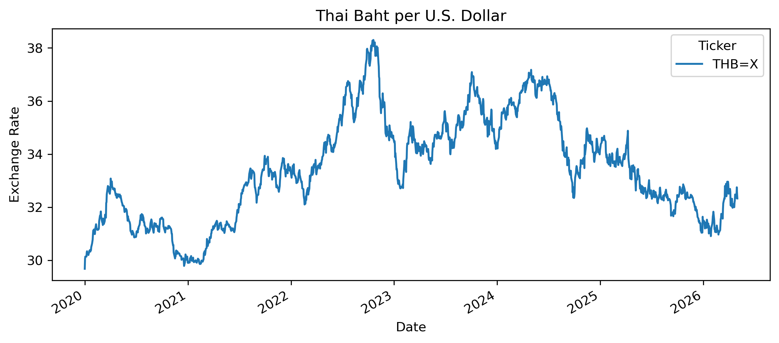
1.13 Gretl Example: Opening and Plotting Data
GRETL provides a simple way to visualize time series data.
Step 1: Open a Dataset
Menu:
File → Open data
Choose a dataset.
[GRETL Screenshot Placeholder: Opening data file]Step 2: Plot a Variable
Select a variable and choose:
Variable → Time series plot
[GRETL Screenshot Placeholder: Time series plot]Step 3: Inspect the Graph
Look for:
trends
cycles
volatility
sudden changes
unusual observations
1.14 Structure of This Book
This book gradually develops the main tools of applied time series analysis.
Part I — Data, Uncertainty, and Financial Returns
We begin with financial data, returns, and statistical foundations.
Part II — Seeing Patterns in Time Series
We study visualization, smoothing, and trading indicators.
Part III — Core Time Series Concepts
We introduce:
stationarity
autocorrelation
unit roots
differencing
Part IV — Linear Time Series Models
We study:
AR models
MA models
ARMA models
ARIMA models
Part V — Forecasting
We develop forecasting methods and forecast evaluation.
Part VI — Relationships Between Time Series
We study:
spurious regression
dynamic models
Granger causality
cointegration
error correction models
Part VII — Multivariate Models
We introduce:
VAR models
impulse response functions
VECM
Part VIII — Volatility
We study:
ARCH models
GARCH models
volatility dynamics
1.15 Common Mistakes
1.16 Looking Ahead
This chapter introduced the basic idea of time series analysis and why it matters.
In the next chapter, we turn to financial data and returns.
We will study:
prices versus returns
simple and log returns
compounding
adjusted prices
volatility
stylized facts of financial data
Key Takeaways
Concept Check
Basic
What is a time series?
Give two examples of time series in economics.
Give two examples of time series in finance.
Intuition
How is a time series different from cross-sectional data?
Why does the order of observations matter in time series data?
Why might past values help predict future values?
Intermediate
What is meant by “dependence over time”?
Why might ignoring time structure lead to incorrect conclusions?
Why are time series especially important for forecasting?
Challenge
Suppose two time series both show an upward trend over time.
Does this necessarily mean they are related?
Why or why not?
Interpretation & Practice
Consider a time series of monthly inflation rates.
What does each observation represent?
What does the time index represent?
You are given a plot of a stock price that steadily increases over time.
What feature of the data stands out?
Why might this be important for analysis?
Suppose GDP increases every year for 20 years.
What kind of pattern does this suggest?
Why might this create problems for simple regression analysis?
A student says:
“We can treat time series data just like any other dataset.”
Do you agree or disagree?
Give one reason to support your answer.
Consider two variables:
global GDP
global energy consumption
Both increase over time.
Would you expect a strong correlation?
Does this necessarily imply a meaningful relationship?
Challenge
Suppose you observe a time series where shocks seem to persist over time.
What might this imply about the underlying process?
How might this affect forecasting?