Chapter 12 — Moving Average Models
In the previous chapter, we studied autoregressive (AR) models, where the current value depends on past values of the series itself.
We now turn to another important class of time series models:
This distinction is extremely important:
AR models describe persistence through past values
MA models describe dependence through past disturbances
Together, AR and MA models form the foundation of Box–Jenkins time series analysis.
Learning Objectives
By the end of this chapter, you should be able to:
distinguish MA models from moving-average smoothing
understand the intuition behind MA() processes
derive the mean and variance of MA(1)
understand the autocorrelation structure
interpret ACF and PACF patterns
understand invertibility intuitively
estimate MA models
12.1 Moving Average Smoothing vs MA(q) Models
Earlier, we studied moving average smoothing:
This is a filtering method.
In MA models, the current value is driven by:
current shocks
past shocks
12.2 The Basic Idea
MA models capture how shocks affect the system for several periods.
Examples:
policy shocks affecting output
financial news impacting markets
supply disruptions affecting inflation
12.3 The MA(1) Model
where:
controls the effect of past shocks
12.4 Intuition Behind MA(1)
Unlike AR models:
MA models do NOT depend on past values
they depend on past disturbances
12.5 Simulating MA(1)
Source
import numpy as np
import matplotlib.pyplot as plt

np.random.seed(123)

n = 400
w = np.random.normal(size=n)

theta_values = [0.3, 0.8, -0.8]

fig, ax = plt.subplots(3,1, figsize=(10,8))

for i, theta in enumerate(theta_values):

    x = np.zeros(n)

    for t in range(1,n):
        x[t] = w[t] + theta*w[t-1]

    ax[i].plot(x)
    ax[i].set_title(rf"MA(1), $\theta={theta}$")

plt.tight_layout()
plt.savefig("figs/ch12/ma1.png", dpi=300, bbox_inches="tight")
plt.close()   # replace with plt.show()
12.6 Mean
(assuming zero mean shocks)
12.7 Variance
12.8 Autocovariance
12.9 Autocorrelation Function (ACF)
Simulation
Source
from statsmodels.graphics.tsaplots import plot_acf

plot_acf(x, lags=20)

plt.savefig("figs/ch12/acf.png", dpi=300, bbox_inches="tight")
plt.close()   # replace with plt.show()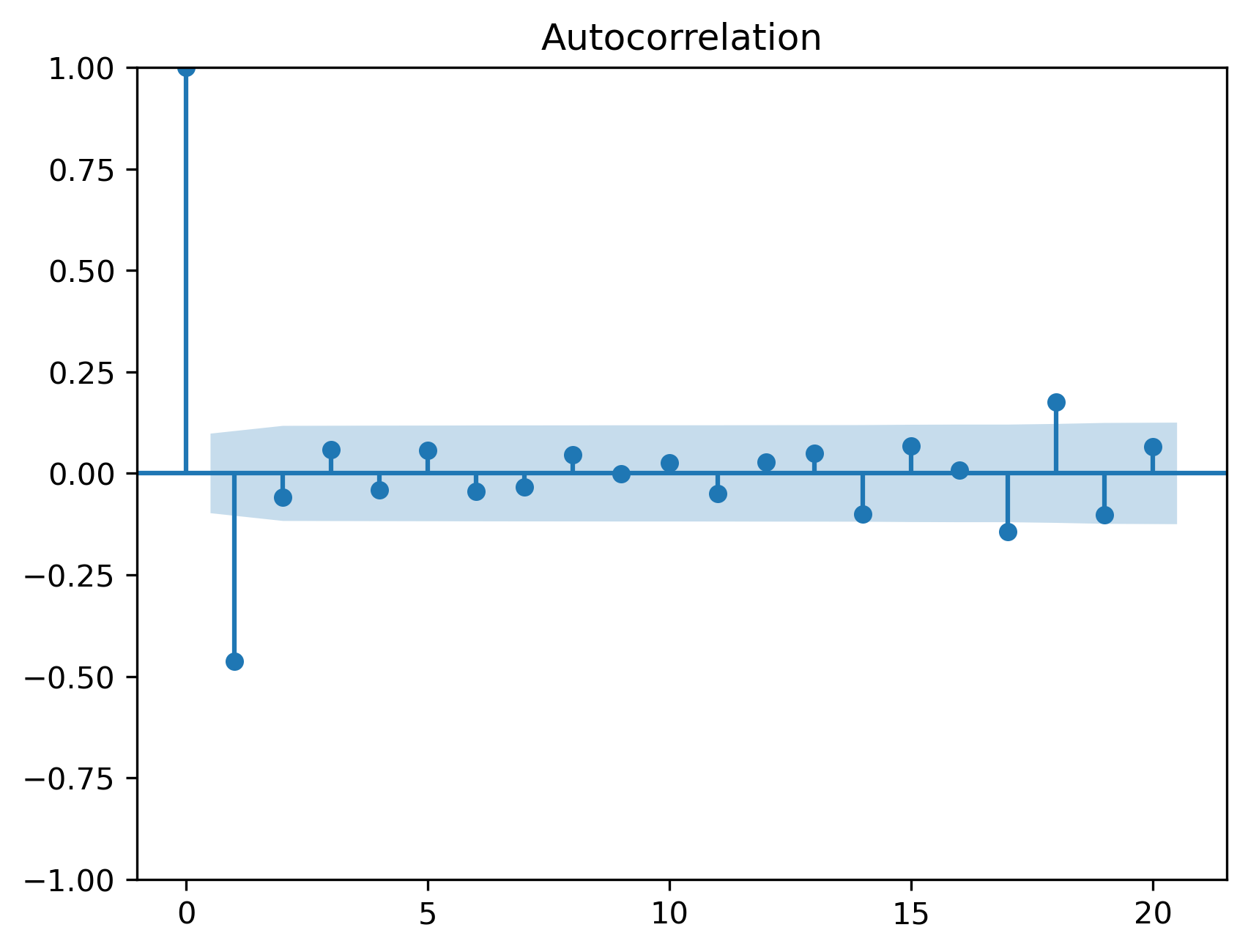
12.10 Partial Autocorrelation (PACF)
Source
from statsmodels.graphics.tsaplots import plot_pacf

plot_pacf(x, lags=20)

plt.savefig("figs/ch12/pacf.png", dpi=300, bbox_inches="tight")
plt.close()   # replace with plt.show()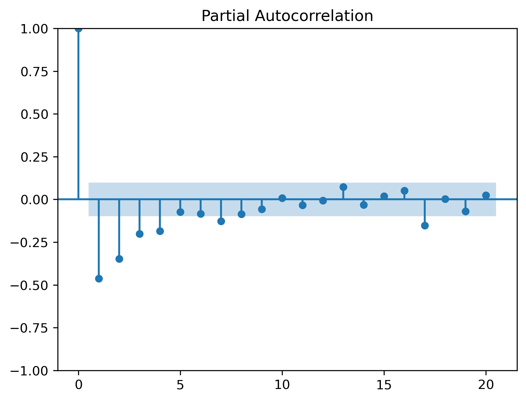
12.11 MA(2)
12.12 General MA(q)
12.13 Invertibility
12.14 AR vs MA
| Feature | AR | MA |
|---|---|---|
| Depends on | past values | past shocks |
| Memory | infinite | finite |
| ACF | tails off | cuts off |
| PACF | cuts off | tails off |
12.15 Estimation
Source
import statsmodels.api as sm

model = sm.tsa.ARIMA(x, order=(0,0,1))
res = model.fit()

print(res.summary())
SARIMAX Results
==============================================================================
Dep. Variable: y No. Observations: 400
Model: ARIMA(0, 0, 1) Log Likelihood -565.364
Date: Mon, 04 May 2026 AIC 1136.727
Time: 21:54:51 BIC 1148.702
Sample: 0 HQIC 1141.469
- 400
Covariance Type: opg
==============================================================================
coef std err z P>|z| [0.025 0.975]
------------------------------------------------------------------------------
const -0.0099 0.010 -0.954 0.340 -0.030 0.010
ma.L1 -0.7942 0.032 -24.900 0.000 -0.857 -0.732
sigma2 0.9865 0.070 14.130 0.000 0.850 1.123
===================================================================================
Ljung-Box (L1) (Q): 0.06 Jarque-Bera (JB): 0.29
Prob(Q): 0.80 Prob(JB): 0.86
Heteroskedasticity (H): 0.69 Skew: 0.07
Prob(H) (two-sided): 0.03 Kurtosis: 3.00
===================================================================================12.16 Diagnostics
Source
from statsmodels.stats.diagnostic import acorr_ljungbox

acorr_ljungbox(res.resid, lags=[10,20], return_df=True)
| | lb_stat | lb_pvalue |
|---------|------------|-----------|
| 10 | 4.539711 | 0.919734 |
| 20 | 23.589777 | 0.260771 |
12.17 Common Mistakes
12.18 Looking Ahead
Next, we combine AR and MA models into ARMA models.
Key Takeaways
Concept Check
Basic
What is a moving average (MA) model?
What is the key difference between:
moving average smoothing
MA() stochastic models
Intuition
In an MA(1) model, how long does a shock affect the system?
What does it mean for an MA process to have finite memory?
How does the parameter affect the behavior of the series?
Intermediate
Why do MA models depend on past shocks rather than past values?
What happens to the effect of a shock after periods in an MA() model?
What is invertibility in MA models?
ACF & PACF
What pattern does the ACF of an MA(1) process exhibit?
What pattern does the PACF of an MA(1) process exhibit?
Why does the ACF “cut off” for MA models?
Finance Insight
Give an example of a real-world situation where shocks have temporary effects.
Why might MA models be useful for modeling short-term market reactions?
Challenge
Suppose is very large (in absolute value).
What might happen to the variability of the series?
Why might invertibility become important?
Interpretation & Practice
A time series reacts strongly to shocks but quickly stabilizes.
What type of model might describe this?
Why?
ACF shows:
large spike at lag 1
near zero afterward
What model is suggested?
PACF shows gradual decay.
What type of model might this indicate?
ACF does NOT cut off sharply.
Why might this happen in practice even if the true model is MA(1)?
A series shows:
temporary reaction to shocks
no long-term persistence
Is this more consistent with AR or MA behavior?
Finance Interpretation
A stock reacts to news for one or two days and then stabilizes.
What type of model could describe this?
Why?
A volatility series shows long-lasting effects of shocks.
Would MA models be sufficient?
Why or why not?
Challenge
A model fits the ACF pattern well but produces poor forecasts.
What might be missing?
Why might combining AR and MA be useful?
Numerical Practice
MA(1) Construction
Consider:
with shocks:
Compute
Comparing Effects
Repeat with:
Compare the magnitude of fluctuations
What changes?
Finite Memory
Suppose a shock of +5 occurs at time in an MA(1).
What is its effect on:
ACF Interpretation
Suppose you observe:
What model is suggested?
Model Identification
You observe:
ACF cuts off after lag 2
PACF decays gradually
What model is suggested?
Estimation Output
Suppose an estimated MA(1) model is:
Is the series highly influenced by past shocks?
How long do shocks persist?
Diagnostics
After estimating an MA model, residuals show:
significant autocorrelation
What does this imply?
What should you do next?
Challenge
Suppose .
Does this violate invertibility?
Why might this be problematic?
Suppose you incorrectly use an MA(1) model when the true process is AR(1).
What patterns might appear in the residuals?
Appendix 12A — Mathematical Details of MA Models
This appendix provides additional insight into the structure of moving average (MA) models.
The goal is to explain why the key results hold, not just state them.
A.1 The MA(1) Process
Consider:
where .
A.2 Mean
Taking expectations:
So:
A.3 Variance
Because shocks are independent:
A.4 Autocovariance
We compute:
Lag 1
Only the shared term ( w_{t-1} ) contributes:
Lag 2
No overlapping shocks:
General Result
A.5 Autocorrelation Function (ACF)
So:
A.6 Why the ACF Cuts Off
This is the defining feature of MA models.
At lag 1:
both and contain
At lag 2:
no common shocks exist
A.7 Invertibility (Deeper Insight)
Consider:
We can rearrange:
Substituting repeatedly:
Thus:
This expresses the MA process as an infinite AR process.
Condition
For convergence:
A.8 Why Invertibility Matters
Without invertibility:
multiple values of produce the same ACF
parameters cannot be uniquely identified
A.9 General MA(q)
Key properties:
ACF cuts off after lag
PACF decays gradually