Part II Capstone — Seeing Patterns and Trading Signals

In Part II, we studied how to see patterns in time series data.

We introduced:

visualization,
trends,
cycles,
noise,
smoothing,
moving averages,
exponential smoothing,
and trading indicators.

This capstone integrates these ideas through a practical applied project using financial price data.

The goal is not to prove that a trading rule works.

The goal is to understand how smoothing and filtering tools transform raw price data into interpretable signals.

Learning Goals¶

By completing this capstone, you should be able to:

visualize financial time series
compute rolling averages
compare short-run and long-run trends
construct basic trading indicators
interpret MACD, RSI, and Bollinger Bands
understand backtesting at a basic level
recognize overfitting and false signals

Dataset¶

We will use the Thai SET Index.

Exercise 1 — Downloading and Plotting the SET Index¶

import yfinance as yf
import matplotlib.pyplot as plt

set_index = yf.download(
    "^SET.BK",
    start="2018-01-01",
    auto_adjust=False
)

prices = set_index["Adj Close"].squeeze()

prices.plot(figsize=(10,4))

plt.title("Thai SET Index Adjusted Closing Prices")
plt.xlabel("Date")
plt.ylabel("Index Level")

plt.savefig("figs/ch6_/set.png", dpi=300, bbox_inches="tight")
plt.close()   # replace with plt.show()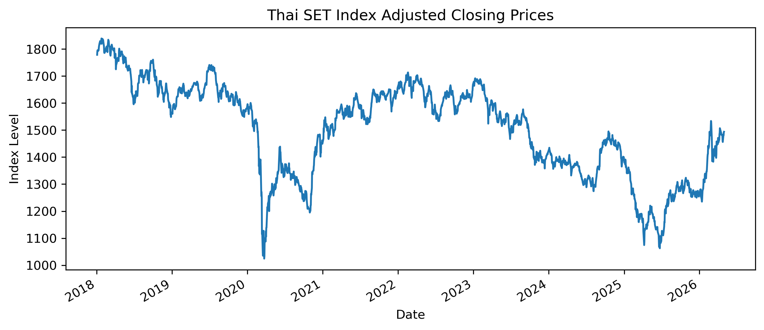

# Save CSV file
set_index.to_csv(
    "figs/ch6_/set.csv")

Questions¶

Does the SET Index display a clear trend?
Can you identify periods of sharp decline?
Are there periods where the series appears especially volatile?

Exercise 2 — Rolling Averages¶

We now compute short-run and long-run moving averages.

ma30 = prices.rolling(30).mean()

ma100 = prices.rolling(100).mean()

plt.figure(figsize=(10,5))

plt.plot(prices, label="SET Index")
plt.plot(ma30, label="30-Day Moving Average")
plt.plot(ma100, label="100-Day Moving Average")

plt.legend()

plt.title("SET Index with Moving Averages")
plt.xlabel("Date")
plt.ylabel("Index Level")

plt.savefig("figs/ch6_/30-100.png", dpi=300, bbox_inches="tight")
plt.close()   # replace with plt.show()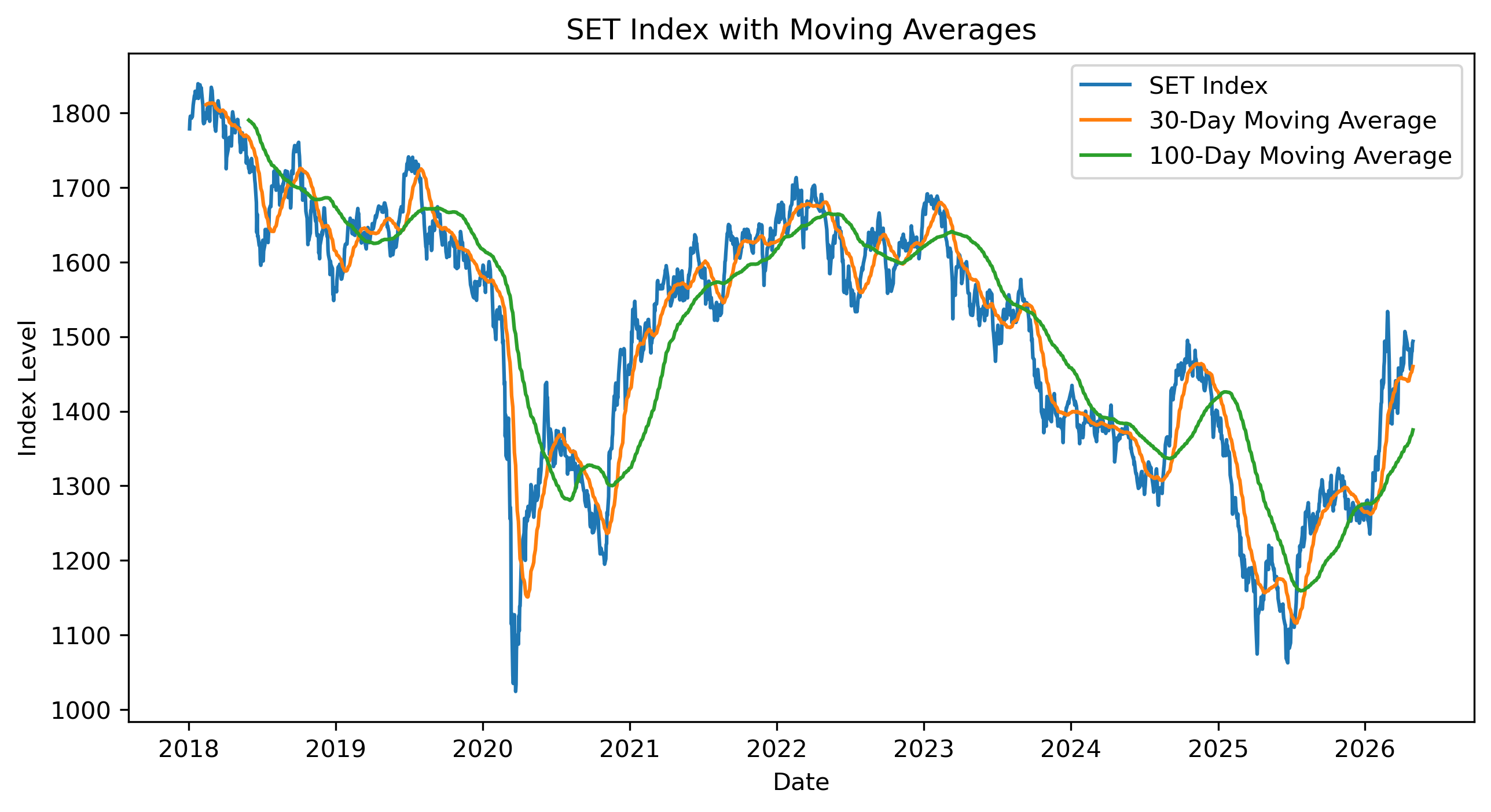

Questions¶

Which moving average responds faster to price changes?
Which moving average is smoother?
What happens to the moving averages during market downturns?

Exercise 3 — Moving Average Crossover Signals¶

A simple trading rule is:

buy when the short moving average is above the long moving average,
stay out of the market otherwise.

import numpy as np
import pandas as pd

signals = pd.DataFrame(index=prices.index)

signals["price"] = prices

signals["ma30"] = ma30

signals["ma100"] = ma100

signals["signal"] = np.where(
    signals["ma30"] > signals["ma100"],
    1,
    0
)

signals["crossover"] = signals["signal"].diff()

signals.tail()

Plotting Buy and Sell Signals¶

buy = signals[signals["crossover"] == 1]

sell = signals[signals["crossover"] == -1]

plt.figure(figsize=(10,5))

plt.plot(signals["price"], label="SET Index")
plt.plot(signals["ma30"], label="30-Day MA")
plt.plot(signals["ma100"], label="100-Day MA")

plt.scatter(
    buy.index,
    buy["price"],
    marker="^",
    s=100,
    label="Buy Signal"
)

plt.scatter(
    sell.index,
    sell["price"],
    marker="v",
    s=100,
    label="Sell Signal"
)

plt.legend()

plt.title("Moving Average Crossover Signals")
plt.xlabel("Date")
plt.ylabel("Index Level")

plt.savefig("figs/ch6_/MAC.png", dpi=300, bbox_inches="tight")
plt.close()   # replace with plt.show()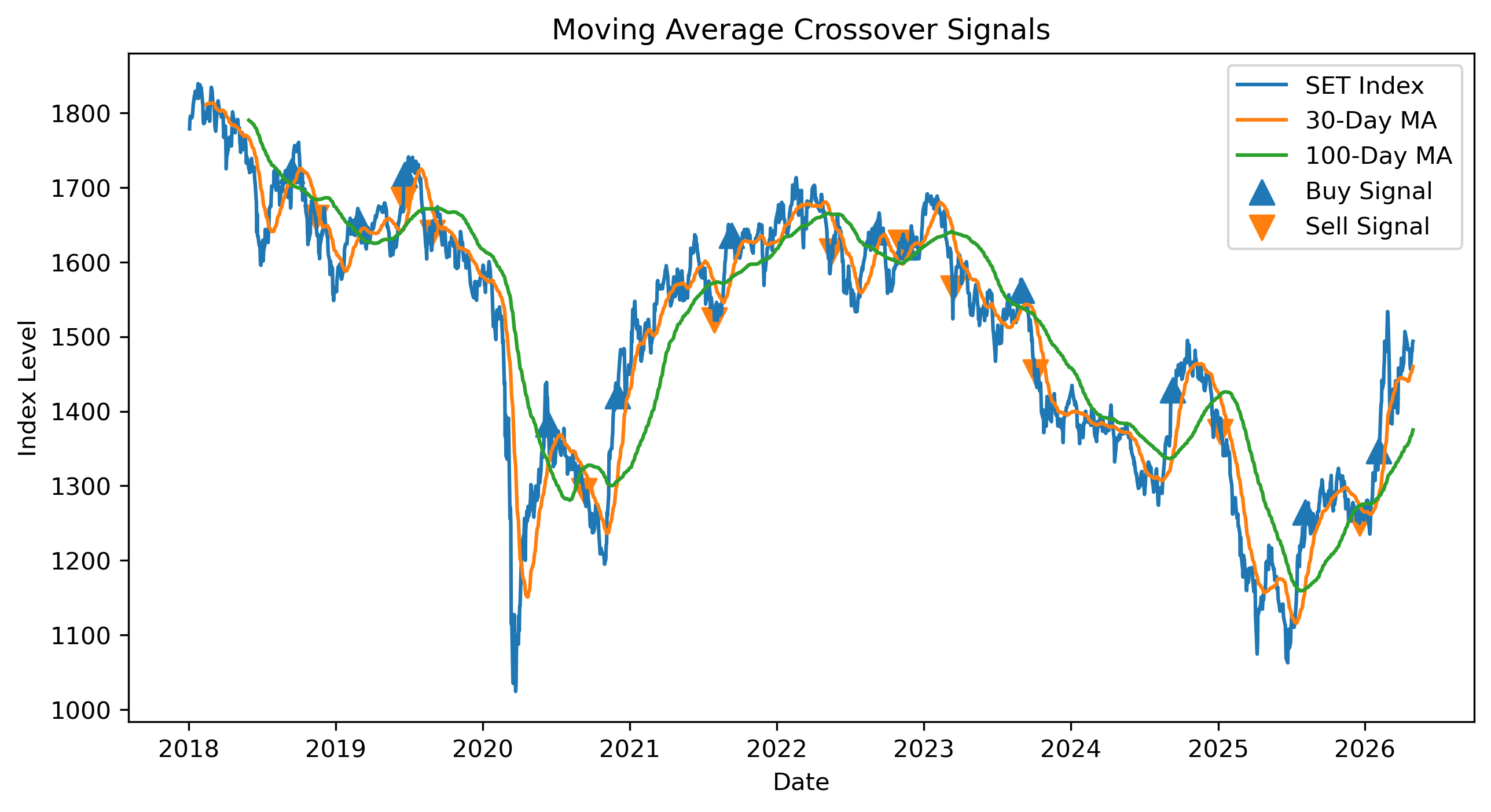

Questions¶

Do the buy signals appear early or late?
Do the sell signals appear early or late?
What are the advantages and disadvantages of using moving average crossovers?

Exercise 4 — MACD¶

MACD compares short-run and long-run exponential moving averages.

ema12 = prices.ewm(
    span=12,
    adjust=False
).mean()

ema26 = prices.ewm(
    span=26,
    adjust=False
).mean()

macd = ema12 - ema26

signal_line = macd.ewm(
    span=9,
    adjust=False
).mean()

plt.figure(figsize=(10,5))

plt.plot(macd, label="MACD")
plt.plot(signal_line, label="Signal Line")

plt.axhline(
    0,
    linestyle="--",
    linewidth=1
)

plt.legend()

plt.title("MACD Indicator")
plt.xlabel("Date")

plt.savefig("figs/ch6_/MACD.png", dpi=300, bbox_inches="tight")
plt.close()   # replace with plt.show()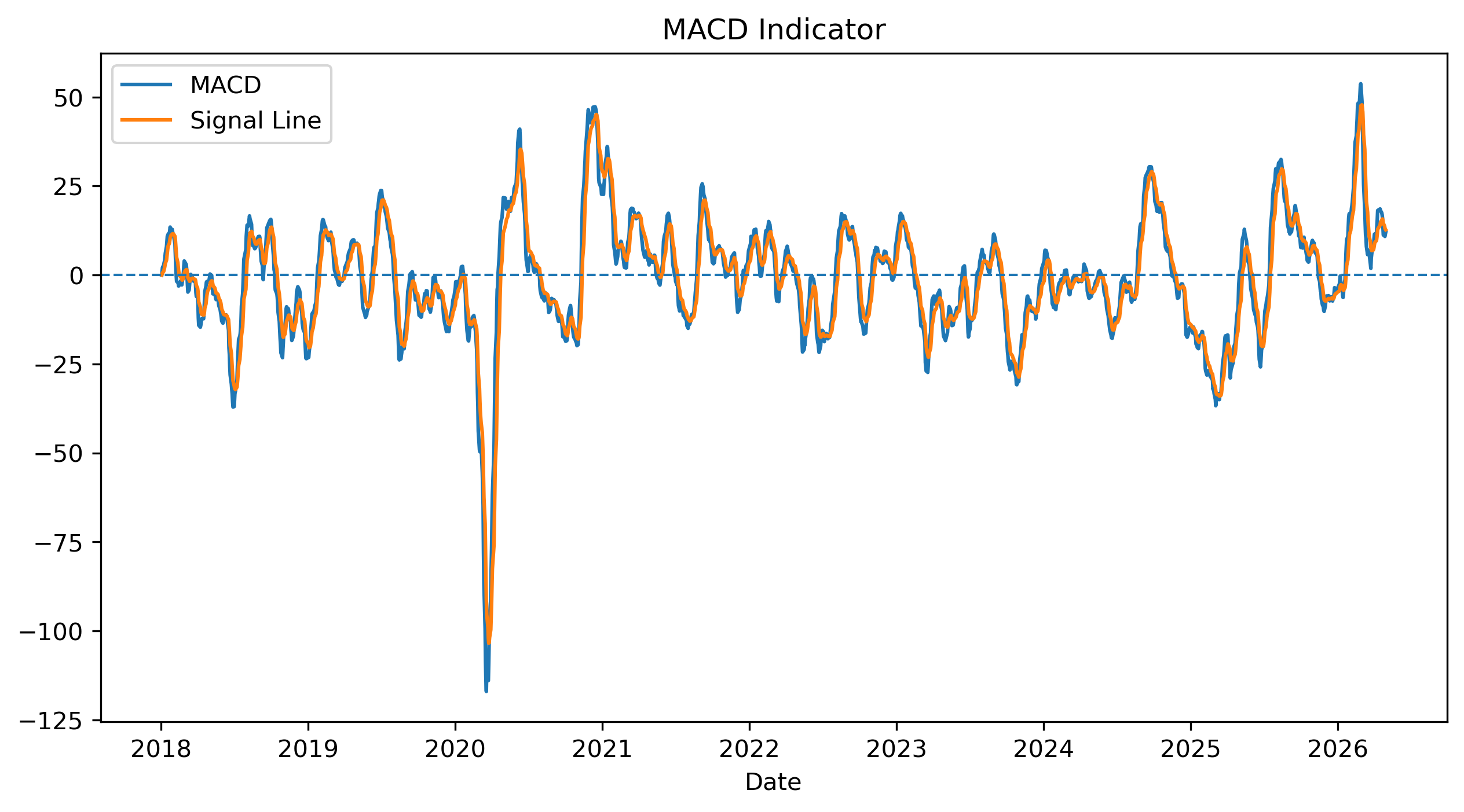

Questions¶

How does MACD differ from the simple moving average crossover?
Does MACD react faster or slower than the 50/200 moving average rule?
Can you identify false signals?

Exercise 5 — RSI¶

RSI attempts to identify overbought and oversold conditions.

delta = prices.diff()

up = delta.clip(lower=0)

down = -delta.clip(upper=0)

roll_up = up.rolling(14).mean()

roll_down = down.rolling(14).mean()

rs = roll_up / roll_down

rsi = 100 - (100 / (1 + rs))

plt.figure(figsize=(10,4))

plt.plot(rsi, label="RSI")

plt.axhline(
    70,
    linestyle="--",
    linewidth=1,
    label="Overbought"
)

plt.axhline(
    30,
    linestyle="--",
    linewidth=1,
    label="Oversold"
)

plt.legend()

plt.title("Relative Strength Index (RSI)")
plt.xlabel("Date")

plt.savefig("figs/ch6_/rsi.png", dpi=300, bbox_inches="tight")
plt.close()   # replace with plt.show()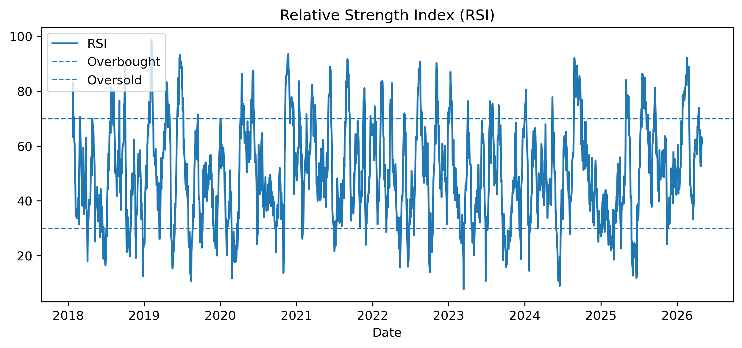

Questions¶

When does RSI move above 70?
When does RSI move below 30?
Does an overbought signal always imply that prices will fall immediately?

Exercise 6 — Bollinger Bands¶

Bollinger Bands combine smoothing and volatility.

ma50 = prices.rolling(50).mean()

std50 = prices.rolling(50).std()

upper = ma50 + 2 * std50

lower = ma50 - 2 * std50

plt.figure(figsize=(10,5))

plt.plot(prices, label="SET Index")
plt.plot(ma50, label="50-Day MA")
plt.plot(upper, label="Upper Band")
plt.plot(lower, label="Lower Band")

plt.legend()

plt.title("Bollinger Bands")
plt.xlabel("Date")
plt.ylabel("Index Level")

plt.savefig("figs/ch6_/BB.png", dpi=300, bbox_inches="tight")
plt.close()   # replace with plt.show()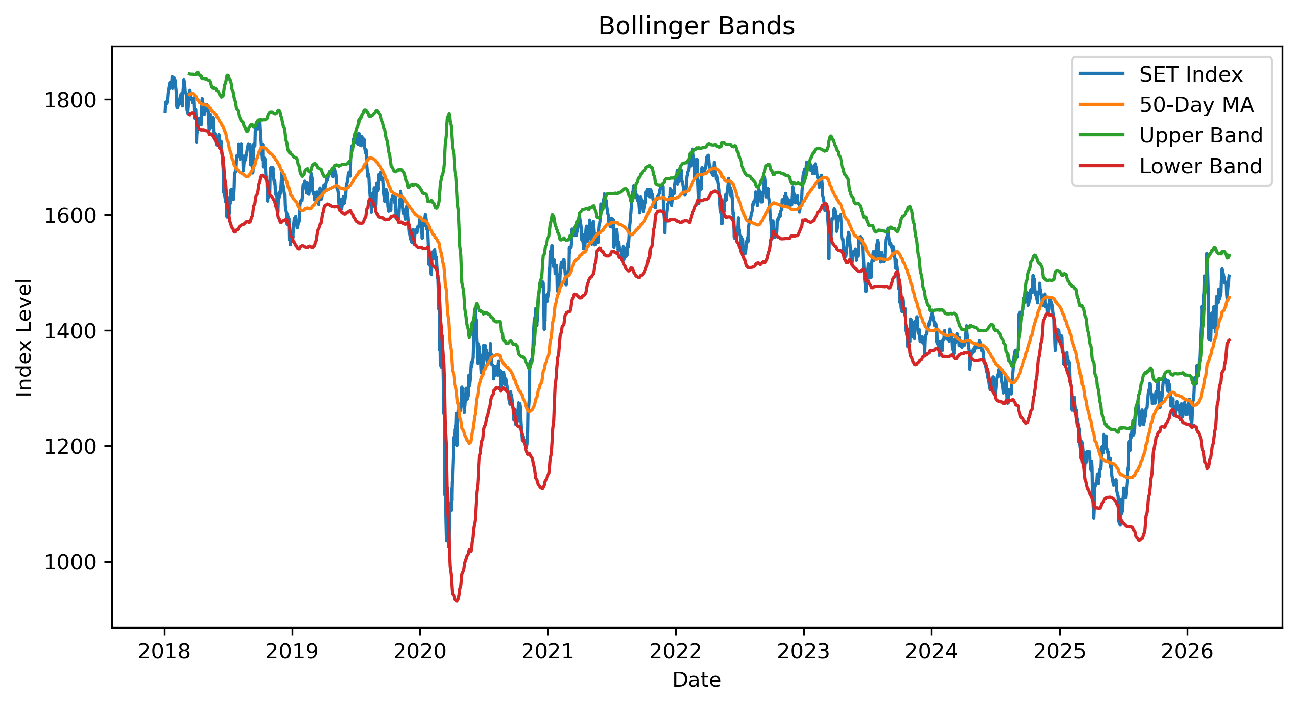

Questions¶

When do the bands become wider?
What does it mean when prices move outside the bands?
Why are Bollinger Bands related to volatility?

Exercise 7 — A Very Simple Backtest¶

We now evaluate a simple moving average strategy.

The strategy is:

hold the market when the 30-day moving average is above the 100-day moving average,
otherwise hold cash.

returns = prices.pct_change()

strategy_position = signals["signal"].shift(1)

strategy_returns = strategy_position * returns

comparison = pd.DataFrame(index=prices.index)

comparison["Buy and Hold"] = (1 + returns).cumprod()

comparison["MA Strategy"] = (1 + strategy_returns).cumprod()

comparison.plot(figsize=(10,5))

plt.title("Buy-and-Hold vs Moving Average Strategy")
plt.ylabel("Cumulative Growth")
plt.xlabel("Date")

plt.savefig("figs/ch6_/backtest.png", dpi=300, bbox_inches="tight")
plt.close()   # replace with plt.show()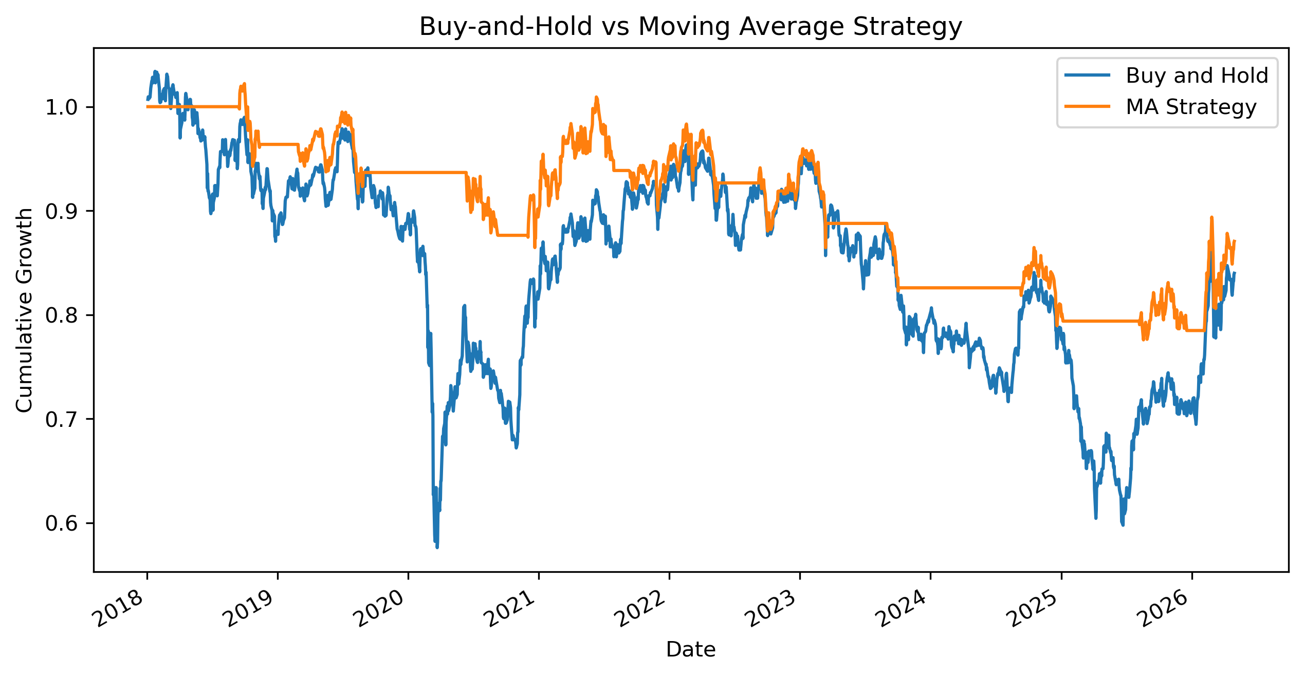

Questions¶

Which strategy performed better over this sample?
Did the moving average strategy reduce losses during downturns?
Did the strategy miss some recoveries?
How might transaction costs affect the result?

Exercise 8 — Comparing Indicators¶

Create a short table summarizing the indicators used in this capstone.

Indicator	Main Idea	Best Suited For
Moving average crossover	trend following	persistent trends
MACD	momentum	trend acceleration
RSI	overbought/oversold	reversal analysis
Bollinger Bands	deviation from average	volatility regimes

Questions¶

Which indicators are trend-following?
Which indicators are closer to mean-reversion logic?
Why might different indicators give conflicting signals?

Mini Project — Your Own Trading Signal Study¶

Choose one asset.

Examples:

SET50,
SPY,
AAPL,
Bitcoin,
Thai baht per U.S. dollar,
gold prices.

Then complete the following tasks:

Download daily price data.
Plot adjusted prices.
Compute 50-day and 200-day moving averages.
Identify crossover signals.
Compute MA cross over.
Compute RSI.
Plot Bollinger Bands.
Conduct a simple backtest using all 3 strategies.
Discuss whether the indicators were useful.

Gretl Version¶

The same ideas can also be explored in Gretl.

Moving Averages¶

Menu:

Add → Moving average

Choose the window length.

Plotting Indicators¶

Menu:

Variable → Time series plot

Then add smoothed series or generated variables.

Creating Returns¶

Menu:

Add → Define new variable

Example:

return = (P - P(-1))/P(-1)

Common Mistakes¶

Looking Ahead¶

Part III turns from visual pattern recognition to formal time series concepts.

We will study:

randomness,
dependence,
stationarity,
autocorrelation,
unit roots,
and differencing.

Part II Capstone — Seeing Patterns and Trading Signals

Learning Goals¶

Dataset¶

Exercise 1 — Downloading and Plotting the SET Index¶

Questions¶

Exercise 2 — Rolling Averages¶

Questions¶

Exercise 3 — Moving Average Crossover Signals¶

Plotting Buy and Sell Signals¶

Questions¶

Exercise 4 — MACD¶

Questions¶

Exercise 5 — RSI¶

Questions¶

Exercise 6 — Bollinger Bands¶

Questions¶

Exercise 7 — A Very Simple Backtest¶

Questions¶

Exercise 8 — Comparing Indicators¶

Questions¶

Mini Project — Your Own Trading Signal Study¶

Gretl Version¶

Moving Averages¶

Plotting Indicators¶

Creating Returns¶

Common Mistakes¶

Looking Ahead¶

Key Takeaways¶