Part VI Capstone — Spurious Regression, Cointegration, and Dynamic Relationships

In Part VI, we studied how relationships between time series can become substantially more complicated when variables are:

persistent,
trending,
and nonstationary.

We introduced:

spurious regression,
dynamic models,
Granger causality,
cointegration,
and error correction models (ECMs).

We learned that standard regression tools may become misleading when applied directly to nonstationary time series.

At the same time, we also saw that some nonstationary variables may still share meaningful long-run equilibrium relationships.

This capstone integrates these ideas through two applied case studies:

a macroeconomic example using U.S. and Mexico GDP,
and a financial example using international ETFs.

The emphasis is practical and intuition-first.

We focus on:

diagnosing nonstationarity,
identifying spurious regression,
testing for cointegration,
estimating dynamic relationships,
constructing spreads,
and interpreting equilibrium adjustment.

Learning Goals¶

By completing this capstone, you should be able to:

recognize the dangers of spurious regression
test for unit roots using the ADF test
distinguish between stationary and nonstationary relationships
perform Engle–Granger cointegration tests
interpret long-run equilibrium relationships
construct and analyze spreads
estimate simple error correction models
understand the logic of pairs trading
distinguish short-run dynamics from long-run equilibrium adjustment
interpret empirical time series relationships carefully

Case A — Does U.S. GDP Help Explain Mexico GDP?¶

Exercise 1 — Download Real GDP Data¶

We begin by downloading quarterly real GDP data for:

the United States,
and Mexico.

We use the FRED database through pandas_datareader.

Downloading GDP Data from FRED¶

import pandas as pd
import pandas_datareader.data as web
import matplotlib.pyplot as plt

usa_gdp = web.DataReader(
    "GDPC1",
    "fred",
    start="1995-01-01"
)

mex_gdp = web.DataReader(
    "NGDPRSAXDCMXQ",
    "fred",
    start="1995-01-01"
)

usa_gdp.columns = ["USA_GDP"]
mex_gdp.columns = ["MEXICO_GDP"]

gdp = pd.concat(
    [usa_gdp, mex_gdp],
    axis=1
).dropna()

gdp.head()

| DATE       | USA_GDP   | MEXICO_GDP |
|------------|-----------|------------|
| 1995-01-01 | 11319.951 | 3519803.5  |
| 1995-04-01 | 11353.721 | 3306332.9  |
| 1995-07-01 | 11450.310 | 3377180.2  |
| 1995-10-01 | 11528.067 | 3454404.3  |
| 1996-01-01 | 11614.418 | 3534597.8  |
...

Exercise 2 — Plot GDP Levels¶

fig, ax1 = plt.subplots(figsize=(10,5))

# ==========================================
# USA GDP
# ==========================================

ax1.plot(
    gdp.index,
    gdp["USA_GDP"],
    linewidth=2,
    label="USA Real GDP"
)

ax1.set_ylabel("USA Real GDP")

# ==========================================
# Mexico GDP
# ==========================================

ax2 = ax1.twinx()

ax2.plot(
    gdp.index,
    gdp["MEXICO_GDP"],
    linewidth=2,
    linestyle="--",
    label="Mexico Real GDP"
)

ax2.set_ylabel("Mexico Real GDP")

# ==========================================
# Title
# ==========================================

plt.title("USA and Mexico Real GDP")

# ==========================================
# Combined legend
# ==========================================

lines1, labels1 = ax1.get_legend_handles_labels()

lines2, labels2 = ax2.get_legend_handles_labels()

ax1.legend(
    lines1 + lines2,
    labels1 + labels2,
    loc="upper left"
)

plt.savefig("figs/ch21_/USA_Mexico.png", dpi=300, bbox_inches="tight")
plt.close()   # replace with plt.show()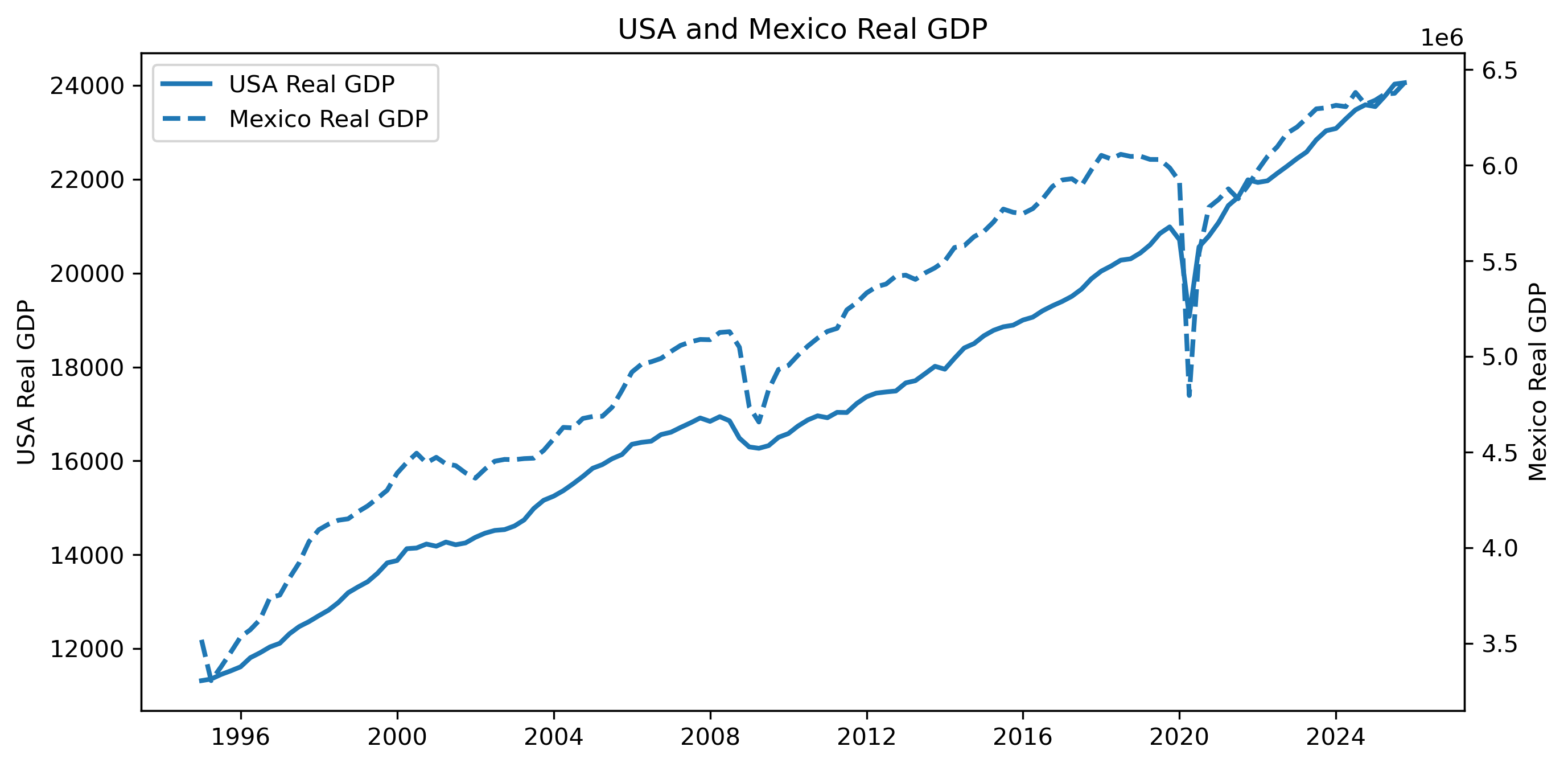

Questions¶

Do the two GDP series appear to move together?
Do both series appear nonstationary?
Could a regression in levels produce misleading results?

Exercise 3 — A Naïve Levels Regression¶

Suppose we regress Mexico real GDP on U.S. real GDP.

import statsmodels.api as sm

# ==========================================
# Regression variables
# ==========================================

y = gdp["MEXICO_GDP"]

X = gdp["USA_GDP"]

X = sm.add_constant(X)

# ==========================================
# Estimate regression
# ==========================================

model = sm.OLS(y, X).fit()

print(model.summary())

                            OLS Regression Results                            
==============================================================================
Dep. Variable:             MEXICO_GDP   R-squared:                       0.947
Model:                            OLS   Adj. R-squared:                  0.946
Method:                 Least Squares   F-statistic:                     2169.
Date:                Sun, 03 May 2026   Prob (F-statistic):           1.50e-79
Time:                        19:52:53   Log-Likelihood:                -1681.8
No. Observations:                 124   AIC:                             3368.
Df Residuals:                     122   BIC:                             3373.
Df Model:                           1                                         
Covariance Type:            nonrobust                                         
==============================================================================
                 coef    std err          t      P>|t|      [0.025      0.975]
------------------------------------------------------------------------------
const        1.07e+06   8.87e+04     12.067      0.000    8.95e+05    1.25e+06
USA_GDP      234.0011      5.024     46.572      0.000     224.055     243.948
==============================================================================
Omnibus:                        8.847   Durbin-Watson:                   0.243
Prob(Omnibus):                  0.012   Jarque-Bera (JB):                8.701
Skew:                          -0.572   Prob(JB):                       0.0129
Kurtosis:                       3.614   Cond. No.                     9.21e+04
==============================================================================

Notes:
[1] Standard Errors assume that the covariance matrix of the errors is correctly specified.
[2] The condition number is large, 9.21e+04. This might indicate that there are
strong multicollinearity or other numerical problems.

Questions¶

Is the estimated relationship statistically significant?
Is the (R^2) large?
Does this necessarily imply a genuine economic relationship?
Why might trending variables create misleading regressions?

Visualizing the Fitted Relationship¶

plt.figure(figsize=(8,5))

# Scatter plot
plt.scatter(
    gdp["USA_GDP"],
    gdp["MEXICO_GDP"],
    alpha=0.7
)

# Fitted regression line
plt.plot(
    gdp["USA_GDP"],
    model.fittedvalues,
    linewidth=2
)

plt.title("Mexico GDP vs USA GDP")

plt.xlabel("USA Real GDP")

plt.ylabel("Mexico Real GDP")

plt.savefig(
    "figs/ch21_/corr.png",
    dpi=300,
    bbox_inches="tight"
)

plt.close()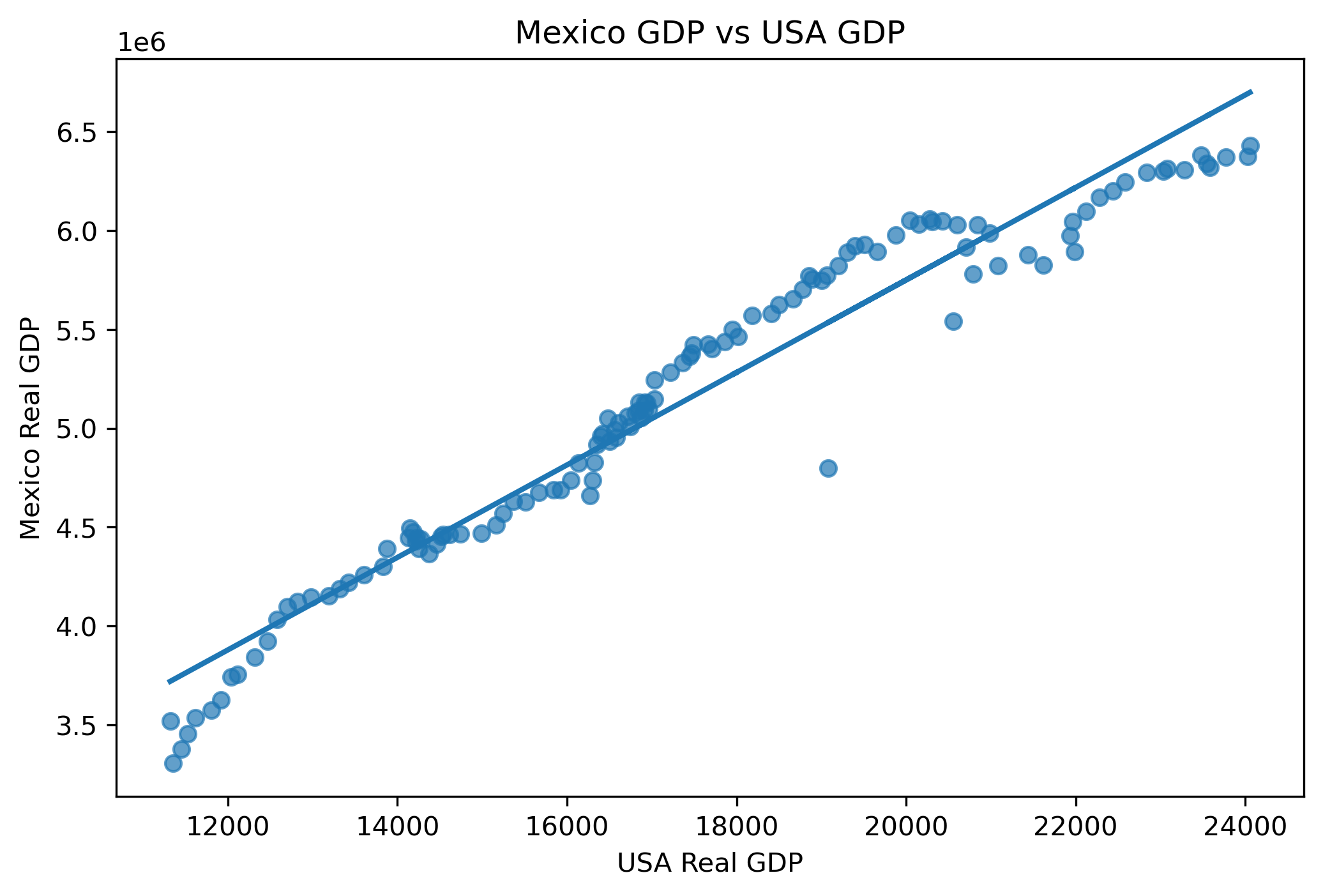

Exercise 4 — Testing for Unit Roots¶

We now investigate whether the GDP series are stationary.

This is crucial because regressions involving nonstationary variables may be misleading.

We use the:

A large p-value means we fail to reject nonstationarity.

ADF Test for USA GDP¶

from statsmodels.tsa.stattools import adfuller

adf_usa = adfuller(
    gdp["USA_GDP"]
)

print("ADF Statistic:", adf_usa[0])

print("p-value:", adf_usa[1])

ADF Statistic: 0.32391792020851595
p-value: 0.9784156046782101

ADF Test for Mexico GDP¶

adf_mex = adfuller(
    gdp["MEXICO_GDP"]
)

print("ADF Statistic:", adf_mex[0])

print("p-value:", adf_mex[1])

ADF Statistic: -1.5738505359705157
p-value: 0.49671453217914335

Questions¶

Are the p-values small or large?
Do we reject the unit root null?
Do the GDP series appear stationary?
Why might macroeconomic variables often contain unit roots?

Exercise 5 — Differencing the Data¶

We now difference the GDP series.

gdp_diff = gdp.diff().dropna()

gdp_diff.head()

| DATE       | USA_GDP  | MEXICO_GDP  |
|------------|----------|-------------|
| 1995-04-01 | 33.770   | -213470.6   |
| 1995-07-01 | 96.589   | 70847.3     |
| 1995-10-01 | 77.757   | 77224.1     |
| 1996-01-01 | 86.351   | 80193.5     |
| 1996-04-01 | 193.722  | 37988.0     |
...

Plotting GDP Differences¶

fig, ax1 = plt.subplots(figsize=(10,5))

# ==========================================
# USA GDP Growth
# ==========================================

ax1.plot(
    gdp_diff.index,
    gdp_diff["USA_GDP"],
    linewidth=2,
    label="USA GDP Difference"
)

ax1.set_ylabel("USA GDP Difference")

# ==========================================
# Mexico GDP Growth
# ==========================================

ax2 = ax1.twinx()

ax2.plot(
    gdp_diff.index,
    gdp_diff["MEXICO_GDP"],
    linewidth=2,
    linestyle="--",
    label="Mexico GDP Difference"
)

ax2.set_ylabel("Mexico GDP Difference")

# ==========================================
# Title
# ==========================================

plt.title("Differenced GDP Series")

# ==========================================
# Combined Legend
# ==========================================

lines1, labels1 = ax1.get_legend_handles_labels()

lines2, labels2 = ax2.get_legend_handles_labels()

ax1.legend(
    lines1 + lines2,
    labels1 + labels2,
    loc="upper left"
)

plt.savefig("figs/ch21_/diff.png", dpi=300, bbox_inches="tight")
plt.close()   # replace with plt.show()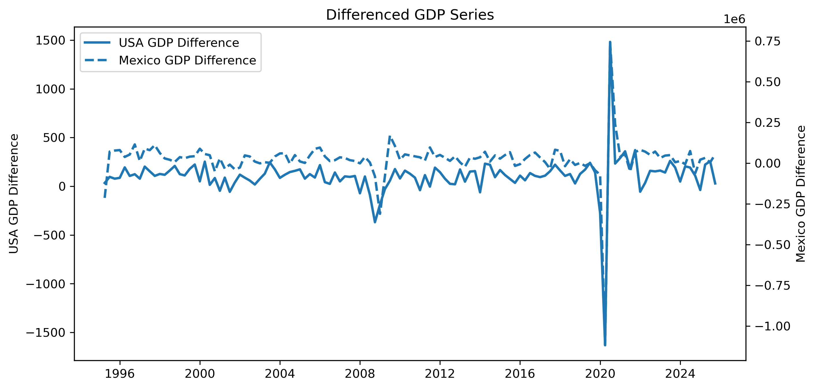

Exercise 6 — ADF Tests on Differenced GDP¶

We now test whether the differenced series are stationary.

USA GDP Differences¶

adf_usa_diff = adfuller(
    gdp_diff["USA_GDP"]
)

print("ADF Statistic:", adf_usa_diff[0])

print("p-value:", adf_usa_diff[1])

ADF Statistic: -13.278665554999852
p-value: 7.772135998540502e-25

Mexico GDP Differences¶

adf_mex_diff = adfuller(
    gdp_diff["MEXICO_GDP"]
)

print("ADF Statistic:", adf_mex_diff[0])

print("p-value:", adf_mex_diff[1])

ADF Statistic: -9.874336285173483
p-value: 3.9187214400492124e-17

Questions¶

Are the differenced series more stationary?
How do the p-values compare with the level series?
Why does differencing often help remove unit roots?

Exercise 7 — Regression in Differences¶

We now estimate a regression using differenced GDP.

import statsmodels.api as sm

y_diff = gdp_diff["MEXICO_GDP"]

X_diff = gdp_diff["USA_GDP"]

X_diff = sm.add_constant(X_diff)

diff_model = sm.OLS(
    y_diff,
    X_diff
).fit()

print(diff_model.summary())

                            OLS Regression Results                            
==============================================================================
Dep. Variable:             MEXICO_GDP   R-squared:                       0.760
Model:                            OLS   Adj. R-squared:                  0.758
Method:                 Least Squares   F-statistic:                     383.3
Date:                Sun, 03 May 2026   Prob (F-statistic):           2.58e-39
Time:                        19:52:54   Log-Likelihood:                -1539.9
No. Observations:                 123   AIC:                             3084.
Df Residuals:                     121   BIC:                             3089.
Df Model:                           1                                         
Covariance Type:            nonrobust                                         
==============================================================================
                 coef    std err          t      P>|t|      [0.025      0.975]
------------------------------------------------------------------------------
const      -3.059e+04   6627.436     -4.616      0.000   -4.37e+04   -1.75e+04
USA_GDP      524.0910     26.768     19.579      0.000     471.097     577.085
==============================================================================
Omnibus:                        8.204   Durbin-Watson:                   2.057
Prob(Omnibus):                  0.017   Jarque-Bera (JB):               10.558
Skew:                          -0.370   Prob(JB):                      0.00510
Kurtosis:                       4.230   Cond. No.                         273.
==============================================================================

Questions¶

How does this regression differ from the levels regression?
Is the relationship weaker or stronger?
Why might differenced regressions be more reliable statistically?

Exercise 8 — Dynamic Interpretation¶

Even if GDP levels are nonstationary, changes in U.S. GDP may still influence changes in Mexico GDP.

This creates a more meaningful interpretation:

Possible channels include:

trade,
manufacturing supply chains,
exports,
investment,
tourism,
and financial conditions.

Looking Ahead¶

We now face an important question:

This leads naturally to:

cointegration,
error correction models,
and dynamic adjustment.

We study these next.

Case B — Cointegration and Pairs Trading¶

Exercise 9 — Download ETF Price Data¶

We now examine two international equity ETFs:

EWA — Australia ETF
EWC — Canada ETF

These economies share several structural similarities:

resource dependence,
commodity exposure,
sensitivity to global growth,
and strong integration into global financial markets.

This makes them plausible candidates for long-run co-movement.

import yfinance as yf
import pandas as pd
import matplotlib.pyplot as plt

ewa = yf.download(
    "EWA",
    start="2015-01-01",
    auto_adjust=False
)

ewc = yf.download(
    "EWC",
    start="2015-01-01",
    auto_adjust=False
)

ewa_prices = ewa["Adj Close"].squeeze()

ewc_prices = ewc["Adj Close"].squeeze()

etf = pd.concat(
    [ewa_prices, ewc_prices],
    axis=1
)

etf.columns = [
    "EWA",
    "EWC"
]

etf = etf.dropna()

etf.head()

| Date       | EWA       | EWC       |
|------------|-----------|-----------|
| 2015-01-02 | 13.892484 | 22.766466 |
| 2015-01-05 | 13.760471 | 22.155445 |
| 2015-01-06 | 13.703897 | 21.830097 |
| 2015-01-07 | 13.829621 | 21.853903 |
| 2015-01-08 | 14.011924 | 22.123701 |
...

Exercise 10 — Plot the Two Price Series¶

indexed = 100 * etf / etf.iloc[0]

indexed.plot(figsize=(10,5))

plt.title("EWA and EWC Indexed Prices")

plt.ylabel("Index (Start = 100)")

plt.savefig("figs/ch21_/ewa_ewc.png", dpi=300, bbox_inches="tight")
plt.close()   # replace with plt.show()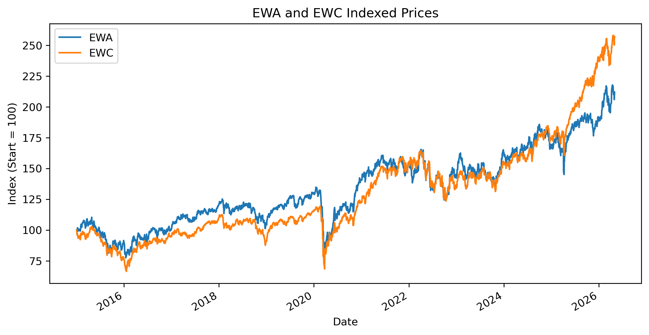

Exercise 11 — Testing ETF Prices for Unit Roots¶

Before testing for cointegration, we must first determine whether the ETF price series are nonstationary.

We use the:

ADF Test for EWA¶

from statsmodels.tsa.stattools import adfuller

adf_ewa = adfuller(
    etf["EWA"]
)

print("ADF Statistic:", adf_ewa[0])

print("p-value:", adf_ewa[1])

ADF Statistic: -0.2498282426693312
p-value: 0.9323156991762888

ADF Test for EWC¶

adf_ewc = adfuller(
    etf["EWC"]
)

print("ADF Statistic:", adf_ewc[0])

print("p-value:", adf_ewc[1])

ADF Statistic: 1.8561991459231966
p-value: 0.9984542009070559

Questions¶

Are the ETF price series stationary?
Are the p-values large or small?
Why are financial price levels often nonstationary?

Exercise 12 — Testing for Cointegration¶

Both ETF price series appear to be nonstationary.

We now ask whether they share a stable long-run relationship.

We use the Engle–Granger cointegration test.

from statsmodels.tsa.stattools import coint

coint_stat, p_value, crit_values = coint(
    etf["EWA"],
    etf["EWC"]
)

print("Cointegration test statistic:", coint_stat)
print("p-value:", p_value)
print("Critical values:", crit_values)

Cointegration test statistic: -2.6696501391297005
p-value: 0.21068363705581145
Critical values: [-3.9002896  -3.33827624 -3.04593952]

Interpretation¶

So:

small p-value → evidence of cointegration
large p-value → little evidence of cointegration

Questions¶

Is the p-value small?
Do we reject the null of no cointegration?
Does the result support the visual impression from the indexed price plot?
Why is cointegration important for pairs trading?

Exercise 13 — Cointegration and Sample Periods¶

Financial relationships may change over time.

We now restrict the sample to:

2015–2024

to investigate whether the apparent divergence after 2025 affects the cointegration result.

etf_sub = etf.loc[
    :"2024-12-31"
]

etf_sub.head()

Plotting the Restricted Sample¶

indexed_sub = 100 * etf_sub / etf_sub.iloc[0]

indexed_sub.plot(figsize=(10,5))

plt.title("EWA and EWC Indexed Prices (2015–2024)")

plt.ylabel("Index (Start = 100)")

plt.savefig("figs/ch21_/ewa_ewc_.png", dpi=300, bbox_inches="tight")
plt.close()   # replace with plt.show()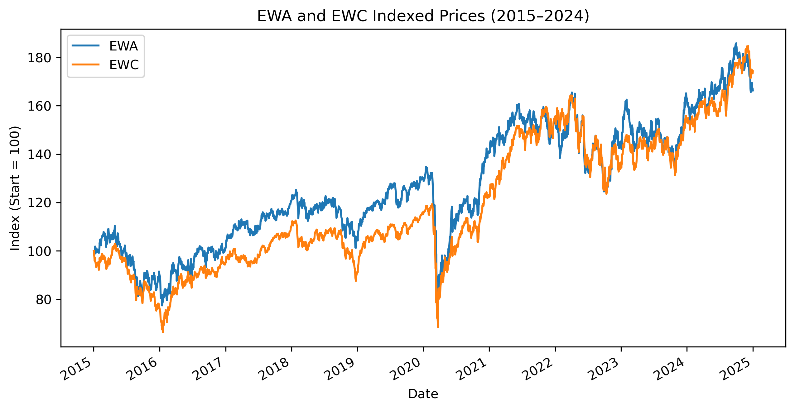

Repeating the Cointegration Test¶

from statsmodels.tsa.stattools import coint

coint_stat, p_value, crit_values = coint(
    etf_sub["EWA"],
    etf_sub["EWC"]
)

print("Cointegration test statistic:", coint_stat)

print("p-value:", p_value)

print("Critical values:", crit_values)

Cointegration test statistic: -3.6441869386563295
p-value: 0.021579983072396378
Critical values: [-3.90079993 -3.33856054 -3.04613679]

Questions¶

Does the cointegration result change?
Why might structural breaks affect cointegration tests?
Why are financial relationships sometimes unstable through time?

Exercise 14 — Estimating the Long-Run Relationship¶

Because the Engle–Granger test suggests evidence of cointegration, we now estimate the long-run equilibrium relationship between:

EWA,
and EWC.

We estimate:

EWA_t = \alpha + \beta EWC_t + u_t

where:

$u_t$ represents deviations from long-run equilibrium.

import statsmodels.api as sm

# ==========================================
# Regression variables
# ==========================================

y = etf_sub["EWA"]

X = etf_sub["EWC"]

X = sm.add_constant(X)

# ==========================================
# Estimate long-run relationship
# ==========================================

longrun_model = sm.OLS(
    y,
    X
).fit()

print(longrun_model.summary())

                            OLS Regression Results                            
==============================================================================
Dep. Variable:                    EWA   R-squared:                       0.961
Model:                            OLS   Adj. R-squared:                  0.961
Method:                 Least Squares   F-statistic:                 6.117e+04
Date:                Sun, 03 May 2026   Prob (F-statistic):               0.00
Time:                        20:51:39   Log-Likelihood:                -2630.8
No. Observations:                2516   AIC:                             5266.
Df Residuals:                    2514   BIC:                             5277.
Df Model:                           1                                         
Covariance Type:            nonrobust                                         
==============================================================================
                 coef    std err          t      P>|t|      [0.025      0.975]
------------------------------------------------------------------------------
const          2.6735      0.062     43.093      0.000       2.552       2.795
EWC            0.5507      0.002    247.316      0.000       0.546       0.555
==============================================================================
Omnibus:                       16.078   Durbin-Watson:                   0.039
Prob(Omnibus):                  0.000   Jarque-Bera (JB):               15.978
Skew:                          -0.179   Prob(JB):                     0.000339
Kurtosis:                       2.844   Cond. No.                         126.
==============================================================================

Questions¶

Is the estimated relationship statistically significant?
What does the slope coefficient imply?
Why should we interpret this relationship cautiously despite evidence of cointegration?

Exercise 15 — Constructing the Spread¶

The residuals from the long-run regression measure deviations from equilibrium.

We define:

\hat u_t = EWA_t - \widehat{\alpha} - \widehat{\beta} EWC_t

This residual series is often called the:

spread = longrun_model.resid

spread.head()

| Date       | Value     |
|------------|-----------|
| 2015-01-02 | -1.319356 |
| 2015-01-05 | -1.114858 |
| 2015-01-06 | -0.992248 |
| 2015-01-07 | -0.879634 |
| 2015-01-08 | -0.845926 |

Plotting the Spread¶

import matplotlib.pyplot as plt

plt.figure(figsize=(10,4))

plt.plot(
    spread,
    linewidth=1.5
)

plt.axhline(
    0,
    linestyle="--",
    linewidth=1
)

plt.title("Cointegration Spread: EWA vs EWC")

plt.ylabel("Spread")

plt.savefig("figs/ch21_/spread.png", dpi=300, bbox_inches="tight")
plt.close()   # replace with plt.show()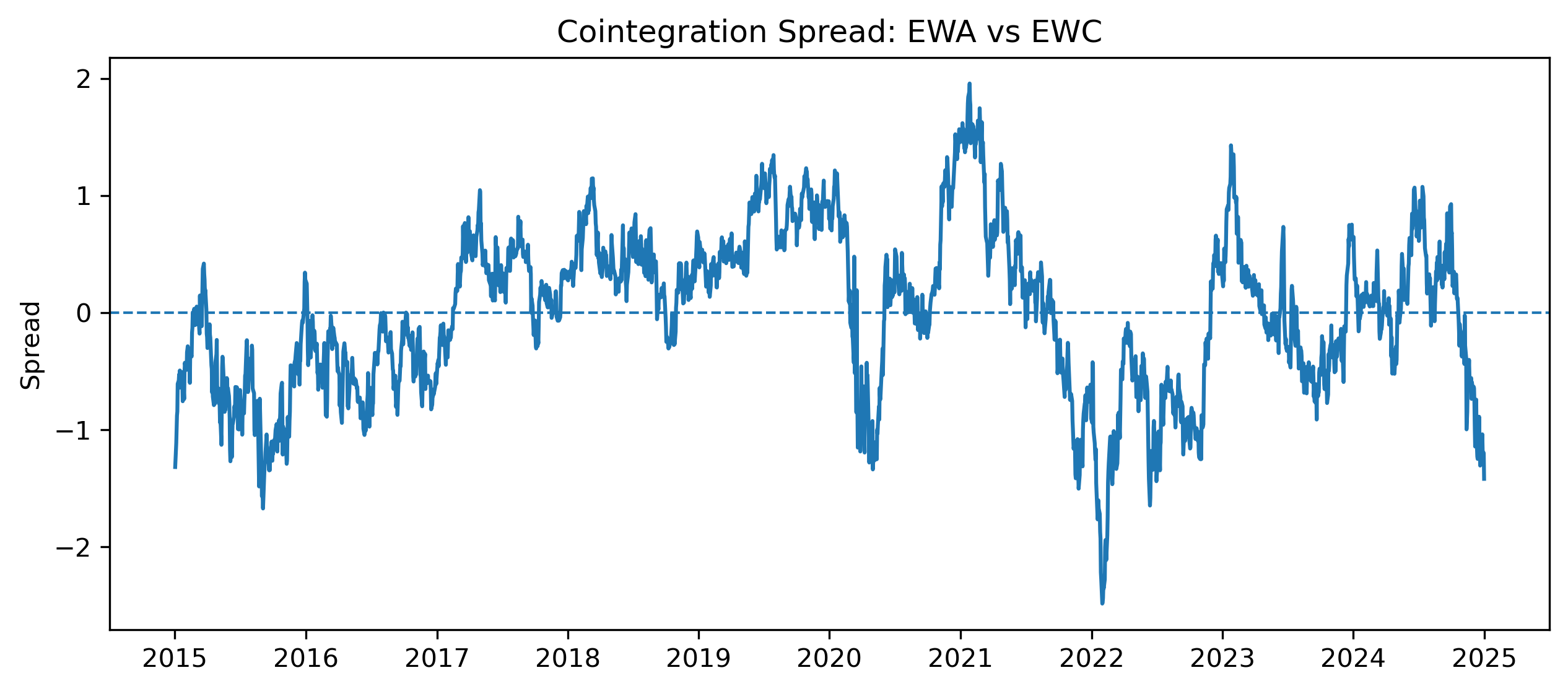

Questions¶

Does the spread appear mean-reverting?
Does the spread fluctuate around zero?
Why is mean reversion important for pairs trading?

Exercise 16 — Testing the Spread for Stationarity¶

We now test whether the spread itself is stationary.

from statsmodels.tsa.stattools import adfuller

spread_adf = adfuller(
    spread
)

print("ADF Statistic:", spread_adf[0])

print("p-value:", spread_adf[1])

ADF Statistic: -3.6414413662018656
p-value: 0.005016429882813343

Questions¶

Is the spread stationary?
Why is spread stationarity central to cointegration?
Why might stationary spreads create trading opportunities?

Exercise 17 — Standardizing the Spread¶

Pairs trading strategies often standardize the spread using a z-score.

spread_mean = spread.mean()

spread_std = spread.std()

zscore = (
    spread - spread_mean
) / spread_std

zscore.head()

Plotting the Z-Score¶

plt.figure(figsize=(10,4))

plt.plot(
    zscore,
    linewidth=1.5
)

plt.axhline(
    2,
    linestyle="--",
    linewidth=1
)

plt.axhline(
    -2,
    linestyle="--",
    linewidth=1
)

plt.axhline(
    0,
    linestyle="--",
    linewidth=1
)

plt.title("Spread Z-Score")

plt.ylabel("Z-Score")

plt.show()

Questions¶

When does the spread appear unusually high?
When does the spread appear unusually low?
Why might traders interpret extreme z-scores as temporary mispricing?

Exercise 18 — A Simple Pairs Trading Rule¶

A very simple rule might be:

Condition	Action
z-score > 2	short spread
z-score < -2	long spread
z-score near 0	close position

Exercise 19 — Estimating an Error Correction Model (ECM)¶

We now model short-run changes together with long-run disequilibrium.

Constructing Differences¶

etf_diff = etf_sub.diff().dropna()

etf_diff.head()

| Date       | EWA      | EWC      |
|------------|----------|----------|
| 2015-01-05 | -0.132009 | -0.611019 |
| 2015-01-06 | -0.056577 | -0.325348 |
| 2015-01-07 |  0.125723 |  0.023808 |
| 2015-01-08 |  0.182301 |  0.269798 |
| 2015-01-09 |  0.132012 | -0.190449 |
...

ECM Estimation¶

We estimate:

\Delta EWA_t = \alpha + \beta \Delta EWC_t + \lambda \hat u_{t-1} + \varepsilon_t

where:

$\hat u_{t-1}$ is the lagged spread.

ecm_data = etf_diff.copy()

ecm_data["spread_lag"] = spread.shift(1)

ecm_data = ecm_data.dropna()

y_ecm = ecm_data["EWA"]

X_ecm = ecm_data[
    ["EWC", "spread_lag"]
]

X_ecm = sm.add_constant(X_ecm)

ecm_model = sm.OLS(
    y_ecm,
    X_ecm
).fit()

print(ecm_model.summary())

                            OLS Regression Results                            
==============================================================================
Dep. Variable:                    EWA   R-squared:                       0.681
Model:                            OLS   Adj. R-squared:                  0.681
Method:                 Least Squares   F-statistic:                     2680.
Date:                Sun, 03 May 2026   Prob (F-statistic):               0.00
Time:                        22:13:47   Log-Likelihood:                 1508.4
No. Observations:                2515   AIC:                            -3011.
Df Residuals:                    2512   BIC:                            -2993.
Df Model:                           2                                         
Covariance Type:            nonrobust                                         
==============================================================================
                 coef    std err          t      P>|t|      [0.025      0.975]
------------------------------------------------------------------------------
const         -0.0005      0.003     -0.200      0.841      -0.006       0.005
EWC            0.6254      0.009     73.139      0.000       0.609       0.642
spread_lag    -0.0201      0.004     -5.217      0.000      -0.028      -0.013
==============================================================================
Omnibus:                      269.386   Durbin-Watson:                   2.328
Prob(Omnibus):                  0.000   Jarque-Bera (JB):             2300.948
Skew:                          -0.022   Prob(JB):                         0.00
Kurtosis:                       7.686   Cond. No.                         3.23
==============================================================================

Questions¶

Is the error correction coefficient statistically significant?
Is the coefficient negative?
Why should the error correction term usually be negative?

Exercise 20 — Economic Interpretation¶

The ECM combines:

short-run dynamics,
and long-run equilibrium adjustment.

This provides a richer interpretation than:

simple correlation,
or static regression.

Questions¶

Why is ECM more appropriate than simple regression for cointegrated series?
Why is cointegration essential before estimating an ECM?
How does the ECM connect finance and time series econometrics?

Synthesis¶

We now contrast the two cases in this capstone.

Case	Main Lesson
USA–Mexico GDP	trending variables may produce spurious regression
EWA–EWC ETFs	nonstationary variables may still share equilibrium relationships

Synthesis Questions¶

Why can GDP levels produce spurious regression?
Why does cointegration change the interpretation?
Why is Granger causality not the same as true causality?
Why is an ECM appropriate only when cointegration exists?
How does pairs trading rely on mean reversion?

Common Mistakes¶

Treating high R² in levels as evidence of a real relationship
Ignoring unit roots
Using ECM without cointegration
Treating Granger causality as structural causality
Backtesting pairs trading without transaction costs

Key Takeaways¶

Relationships between time series require careful diagnosis.
Trending variables can create spurious regression.
Cointegration allows meaningful long-run relationships among nonstationary variables.
Dynamic models capture short-run transmission.
ECMs combine short-run changes with long-run adjustment.

Part C — Pairs Trading with Bollinger Bands on the Spread¶

In the previous section, we estimated the long-run cointegration relationship:

EWA_t = \alpha + \beta EWC_t + u_t

The residual from this equation is the spread:

u_t = EWA_t - \alpha - \beta EWC_t

If the spread is stationary and mean-reverting, unusually large deviations may eventually move back toward equilibrium.

Exercise 21 — Extracting the Hedge Ratio¶

We first extract the estimated intercept and hedge ratio from the long-run regression.

alpha = longrun_model.params["const"]

hedge_ratio = longrun_model.params["EWC"]

print("Alpha:", alpha)

print("Hedge ratio:", hedge_ratio)

Alpha: 2.673501122389125
Hedge ratio: 0.5507372302051009

Exercise 22 — Constructing the Cointegration Spread¶

The spread is:

Spread_t = EWA_t - \alpha - \beta EWC_t

spread = (
    etf_sub["EWA"]
    - alpha
    - hedge_ratio * etf_sub["EWC"]
)

spread.plot(figsize=(10,4))

plt.axhline(
    0,
    linestyle="--",
    linewidth=1
)

plt.title("Cointegration Spread: EWA vs EWC")

plt.ylabel("Spread")

plt.savefig(
    "figs/ch21_/spread_.png",
    dpi=300,
    bbox_inches="tight"
)

plt.savefig("figs/ch21_/spread__.png", dpi=300, bbox_inches="tight")
plt.close()   # replace with plt.show()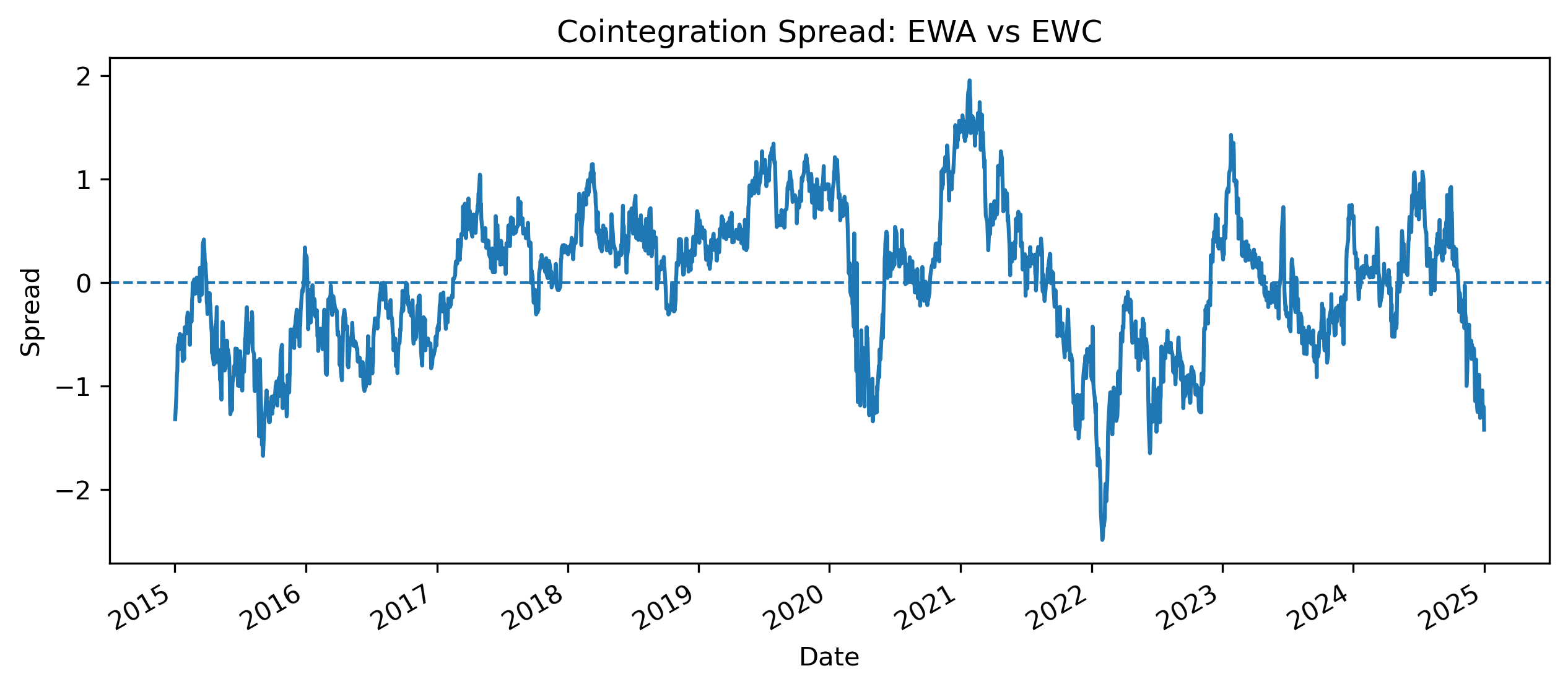

Exercise 23 — Bollinger Bands and Entry Signals on the Spread¶

We now apply Bollinger Bands directly to the cointegration spread.

The bands help identify when the spread is unusually far from its recent average.

window = 20

spread_mean = spread.rolling(window).mean()

spread_std = spread.rolling(window).std()

upper_band = spread_mean + 2 * spread_std

lower_band = spread_mean - 2 * spread_std

Trading Rule¶

Spread condition	Interpretation	Position
spread < lower band	EWA is relatively cheap	Long spread
spread > upper band	EWA is relatively expensive	Short spread
spread returns near mean	equilibrium restored	Close position

Long Spread¶

If:

Spread_t < LowerBand_t

then EWA is relatively cheap.

Short Spread¶

If:

Spread_t > UpperBand_t

then EWA is relatively expensive.

Generating Entry Signals¶

signals = pd.DataFrame(index=spread.index)

signals["spread"] = spread

signals["upper_band"] = upper_band

signals["lower_band"] = lower_band

signals["position"] = 0

# Long spread: buy EWA, short hedge_ratio * EWC
signals.loc[
    signals["spread"] < signals["lower_band"],
    "position"
] = 1

# Short spread: short EWA, buy hedge_ratio * EWC
signals.loc[
    signals["spread"] > signals["upper_band"],
    "position"
] = -1

signals.head()

Plotting the Bands and Entry Signals¶

plt.figure(figsize=(12,5))

plt.plot(
    spread,
    label="Spread",
    linewidth=1.5
)

plt.plot(
    spread_mean,
    label="Rolling Mean",
    linestyle="--"
)

plt.plot(
    upper_band,
    label="Upper Band",
    linestyle=":"
)

plt.plot(
    lower_band,
    label="Lower Band",
    linestyle=":"
)

plt.axhline(
    0,
    linestyle="--",
    linewidth=1
)

long_entries = signals[signals["position"] == 1]

short_entries = signals[signals["position"] == -1]

plt.scatter(
    long_entries.index,
    long_entries["spread"],
    marker="^",
    s=70,
    label="Long Spread Entry"
)

plt.scatter(
    short_entries.index,
    short_entries["spread"],
    marker="v",
    s=70,
    label="Short Spread Entry"
)

plt.legend()

plt.title("Bollinger Bands and Pairs Trading Signals")

plt.ylabel("Spread")

plt.savefig(
    "figs/ch21_/BBspread_signal.png",
    dpi=300,
    bbox_inches="tight"
)

plt.savefig("figs/ch21_/BBspread_signal.png", dpi=300, bbox_inches="tight")
plt.close()   # replace with plt.show()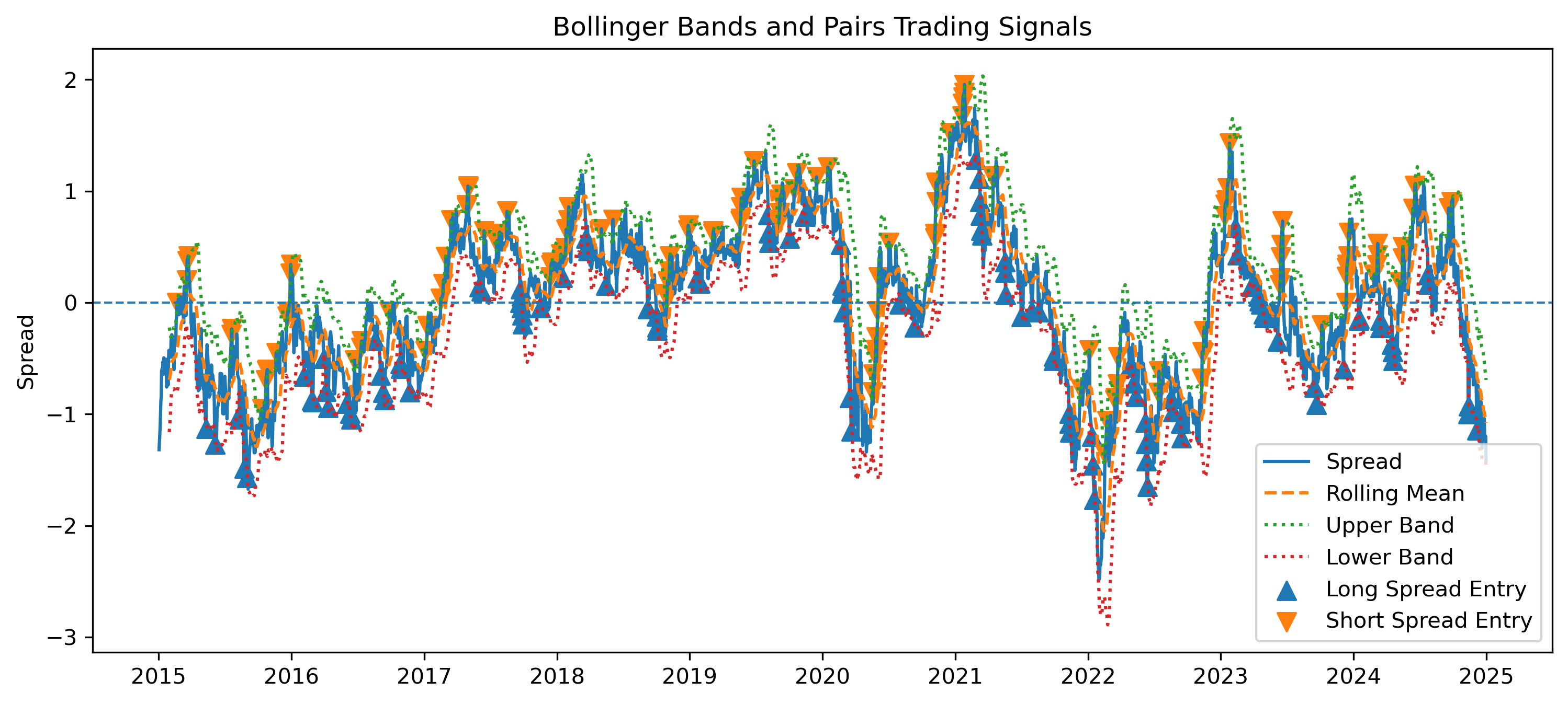

Exercise 24 — Constructing Hedge-Ratio Portfolio Returns¶

We now compute the approximate return from the hedge-ratio pairs strategy.

Recall that the long-run relationship is:

EWA_t = \alpha + \beta EWC_t + u_t

The hedge ratio is:

\beta

So the spread portfolio is:

EWA_t - \beta EWC_t

Strategy Return¶

For a long spread position:

R_t^{long} = R_{EWA,t} - \beta R_{EWC,t}

For a short spread position:

R_t^{short} = - R_{EWA,t} + \beta R_{EWC,t}

This can be written compactly as:

R_t^{strategy} = Position_{t-1} \left( R_{EWA,t} - \beta R_{EWC,t} \right)

where:

$Position_{t-1}=1$ means long spread,
$Position_{t-1}=-1$ means short spread,
$Position_{t-1}=0$ means no position.

Computing Strategy Returns¶

ewa_returns = etf_sub["EWA"].pct_change()

ewc_returns = etf_sub["EWC"].pct_change()

spread_portfolio_returns = (
    ewa_returns
    - hedge_ratio * ewc_returns
)

strategy_position = signals["position"].shift(1)

strategy_returns = (
    strategy_position
    * spread_portfolio_returns
)

strategy_returns = strategy_returns.dropna()

strategy_returns.head()

Questions¶

Why do we use the lagged position rather than the current position?
What does a positive strategy return mean in this context?
Why does the hedge ratio matter for constructing the spread portfolio?
What practical trading costs are ignored in this simple calculation?

Exercise 25 — Backtesting the Pairs Trading Strategy¶

We now evaluate the cumulative performance of the pairs trading strategy.

The goal is to examine whether the strategy was able to profit from mean reversion in the spread.

Cumulative Strategy Performance¶

cumulative_strategy = (
    1 + strategy_returns
).cumprod()

cumulative_strategy.plot(figsize=(10,5))

plt.title("Pairs Trading Strategy Performance")

plt.ylabel("Cumulative Growth")

plt.xlabel("Date")

plt.savefig(
    "figs/ch21_/pairs_backtest.png",
    dpi=300,
    bbox_inches="tight"
)

plt.close()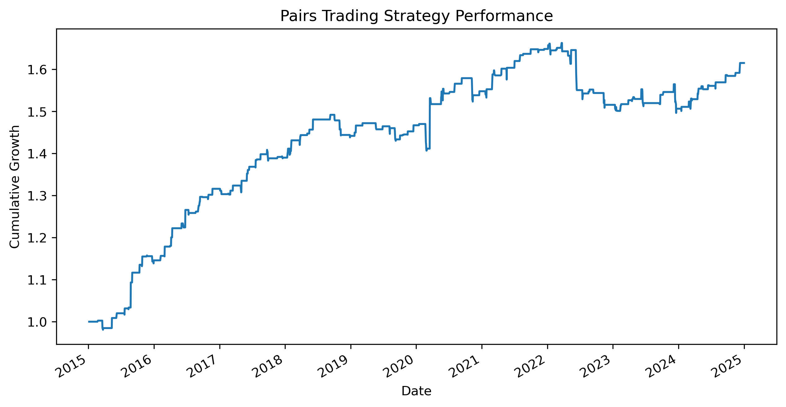

Comparing with Buy-and-Hold¶

We now compare the pairs trading strategy with a simple passive portfolio holding:

50% EWA
50% EWC

This helps illustrate the difference between:

directional investing,
and relative-value investing.

buyhold_returns = (
    0.5 * ewa_returns
    +
    0.5 * ewc_returns
)

buyhold = (
    1 + buyhold_returns
).cumprod()

comparison = pd.concat(
    [
        cumulative_strategy.rename("Pairs Strategy"),
        buyhold.rename("50-50 Buy-and-Hold")
    ],
    axis=1
)

comparison = comparison.dropna()

comparison.plot(figsize=(10,5))

plt.title("Pairs Trading vs 50-50 Buy-and-Hold")

plt.ylabel("Cumulative Growth")

plt.xlabel("Date")

plt.savefig(
    "figs/ch21_/pairs_vs_buyhold.png",
    dpi=300,
    bbox_inches="tight"
)

plt.close()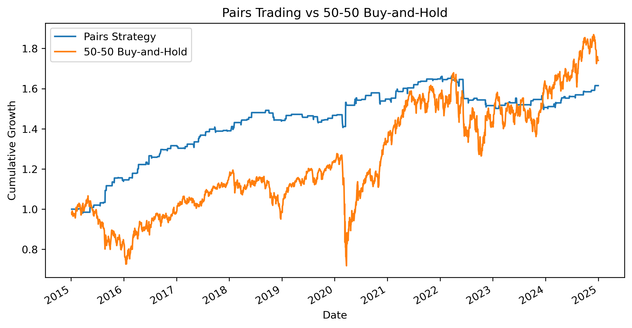

Questions¶

Which strategy appears more stable?
Which strategy experiences larger drawdowns?
Why might a market-neutral strategy behave differently from buy-and-hold investing?
Why might the pairs strategy perform poorly during structural market change?
Does the strategy appear sensitive to the sample period?

Exercise 26 — Evaluating Strategy Risk and Performance¶

Raw returns alone do not fully describe a trading strategy.

We also care about:

volatility,
stability,
drawdowns,
and risk-adjusted performance.

A strategy with high returns but extremely high risk may not be attractive to investors.

Average Daily Return and Volatility¶

We first compute the average daily return and daily volatility of the pairs trading strategy.

mean_return = strategy_returns.mean()

volatility = strategy_returns.std()

print("Average Daily Return:", mean_return)

print("Daily Volatility:", volatility)

Average Daily Return: 0.00019655549078299717
Daily Volatility: 0.003472953960432861

Annualized Performance Measures¶

Because the data are daily, annualized statistics are often easier to interpret and compare.

If:

$\bar R_{daily}$ is the average daily return,
and $\sigma_{daily}$ is the daily volatility,

then the approximate annualized return is:

R_{annual} \approx 252 \times \bar R_{daily}

and the approximate annualized volatility is:

\sigma_{annual} \approx \sqrt{252}\sigma_{daily}

where:

252 approximates the number of trading days in a year.

annual_return = mean_return * 252

annual_volatility = volatility * (252**0.5)

print("Annualized Return:", annual_return)

print("Annualized Volatility:", annual_volatility)

nnualized Return: 0.04953198367731529
Annualized Volatility: 0.055131434964493

Sharpe Ratio¶

A common measure of risk-adjusted performance is the:

which compares:

average return,
relative to volatility.

A simple version is:

Sharpe = \frac{\bar R}{\sigma_R}

where:

$\bar R$ = average return,
$\sigma_R$ = standard deviation of returns.

Daily Sharpe Ratio¶

sharpe = mean_return / volatility

print("Daily Sharpe Ratio:", sharpe)

Daily Sharpe Ratio: 0.056596054258807094

Annualized Sharpe Ratio¶

Because volatility scales with the square root of time, the annualized Sharpe ratio is approximately:

Sharpe_{annual} \approx \sqrt{252} \times Sharpe_{daily}

where:

252 approximates the number of trading days in a year.

annual_sharpe = (252**0.5) * sharpe

print("Annualized Sharpe Ratio:", annual_sharpe)

Annualized Sharpe Ratio: 0.8984345085379295

Comparing with Buy-and-Hold¶

We now compare the volatility of:

the pairs strategy,
and the passive 50-50 buy-and-hold portfolio.

buyhold_volatility = buyhold_returns.std()

buyhold_annual_volatility = (
    buyhold_volatility
    * (252**0.5)
)

print("Pairs Strategy Annualized Volatility:",
      annual_volatility)

print("Buy-and-Hold Annualized Volatility:",
      buyhold_annual_volatility)

Pairs Strategy Annualized Volatility: 0.05513143496449323
Buy-and-Hold Annualized Volatility: 0.20316504936587046

Questions¶

Does the pairs strategy appear less volatile than buy-and-hold?
Why might market-neutral strategies exhibit different risk characteristics?
Is higher return always preferable?
Why are risk-adjusted measures important in finance?
Why might a strategy with lower volatility still be attractive even if raw returns are smaller?

Exercise 27 — Drawdowns and Strategy Stability¶

Average returns and volatility are useful, but they do not show how painful losses can become during bad periods.

A common measure of downside risk is the:

A drawdown measures the percentage decline from a previous peak in cumulative performance.

Computing Drawdowns¶

running_peak = cumulative_strategy.cummax()

drawdown = (
    cumulative_strategy
    / running_peak
    - 1
)

drawdown.plot(figsize=(10,4))

plt.title("Drawdown of Pairs Trading Strategy")

plt.ylabel("Drawdown")

plt.xlabel("Date")

plt.savefig(
    "figs/ch21_/pairs_drawdown.png",
    dpi=300,
    bbox_inches="tight"
)

plt.close()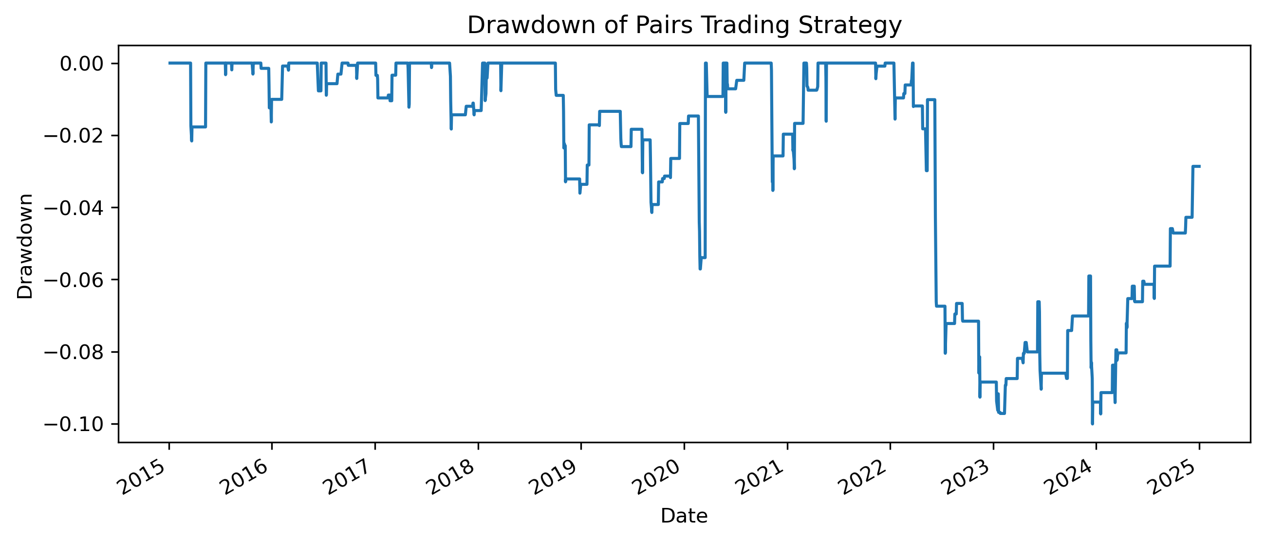

Maximum Drawdown¶

max_drawdown = drawdown.min()

print("Maximum Drawdown:", max_drawdown)

Maximum Drawdown: -0.10007716848807668

Questions¶

When does the largest drawdown occur?
Does the strategy recover quickly from losses?
Why might drawdowns matter more to investors than average returns?
How would transaction costs affect drawdowns?

Exercise 28 — Structural Breakdown and Strategy Instability¶

Earlier, we found that the EWA–EWC cointegration relationship appeared stronger in the 2015–2024 sample, but weaker when later observations were included.

This is a crucial practical lesson.

Extending the Sample¶

We now compare the spread behavior when the sample is extended.

etf_full = etf.copy()

spread_full = (
    etf_full["EWA"]
    - alpha
    - hedge_ratio * etf_full["EWC"]
)

spread_full.plot(figsize=(10,4))

plt.axhline(
    0,
    linestyle="--",
    linewidth=1
)

plt.title("Cointegration Spread Using Extended Sample")

plt.ylabel("Spread")

plt.xlabel("Date")

plt.savefig(
    "figs/ch21_/spread_full_sample.png",
    dpi=300,
    bbox_inches="tight"
)

plt.close()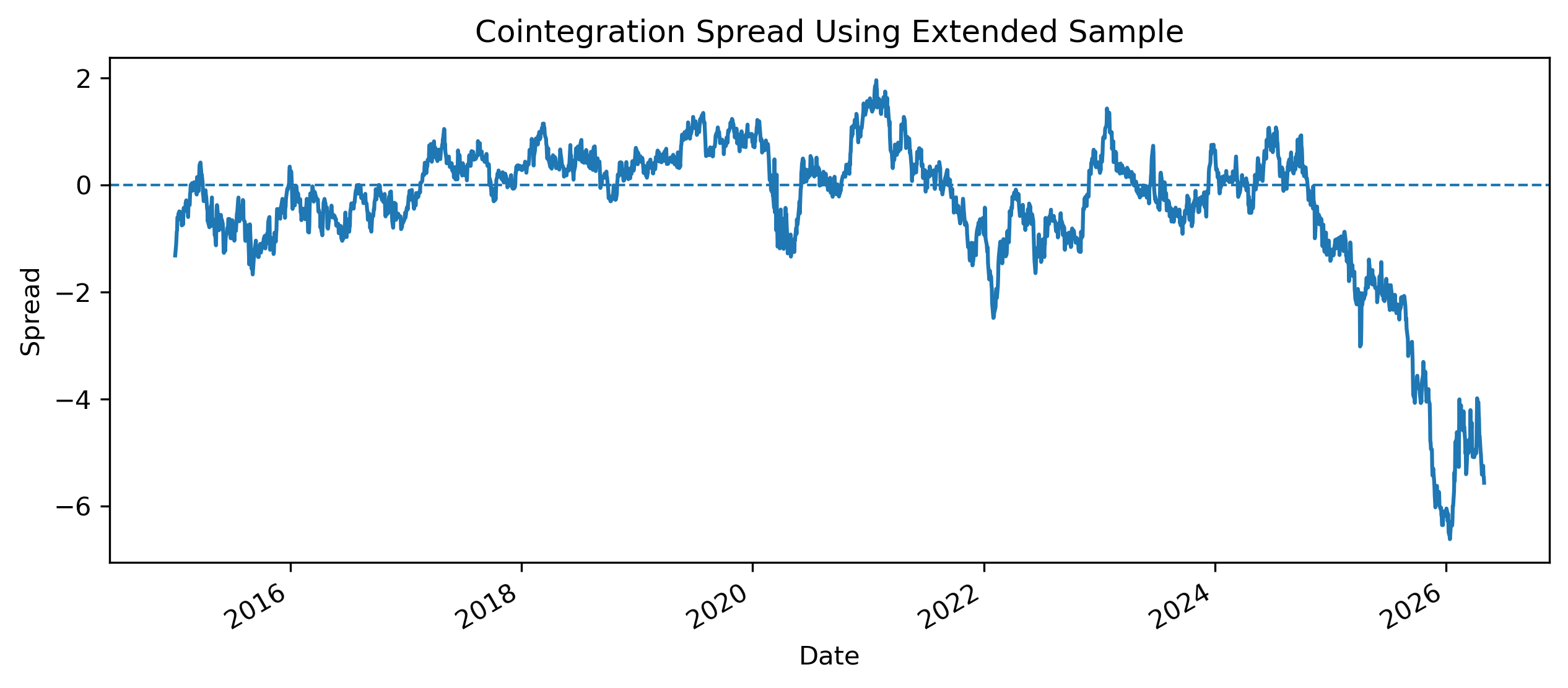

Testing Cointegration in the Extended Sample¶

from statsmodels.tsa.stattools import coint

coint_stat_full, p_value_full, crit_values_full = coint(
    etf_full["EWA"],
    etf_full["EWC"]
)

print("Cointegration test statistic:", coint_stat_full)

print("p-value:", p_value_full)

print("Critical values:", crit_values_full)

Cointegration test statistic: -2.6696490787249836
p-value: 0.21068403165318256
Critical values: [-3.9002896  -3.33827624 -3.04593952]

Questions¶

Does the cointegration result change when the sample is extended?
Does the spread still appear mean-reverting?
Why might financial relationships break down over time?
What would happen to a pairs trading strategy if the spread stopped reverting?

Practical Lessons¶

Possible reasons for structural breakdown include:

changes in commodity exposure,
shifts in monetary policy,
exchange-rate movements,
sector composition changes within ETFs,
changes in global investor behavior,
crisis periods,
and post-sample divergence.

Final Reflection — Equilibrium, Instability, and Financial Markets¶

This capstone illustrates one of the deepest lessons in time series analysis:

In the first case study, U.S. and Mexico GDP appeared strongly related in levels.

The regression produced:

high (R^2),
significant coefficients,
and convincing visual relationships.

Yet nonstationarity created the danger of:

where unrelated trending variables may appear statistically connected.

In the second case study, the EWA and EWC ETFs also displayed strong co-movement.

However, unlike the GDP example, the ETF pair showed evidence of:

meaning that the series appeared linked through a long-run equilibrium relationship.

This allowed us to construct:

spreads,
error correction models,
and pairs trading strategies.

At the same time, the capstone also revealed an important practical reality:

The cointegration relationship became less convincing when the sample period was extended beyond 2024.

This illustrates the importance of:

structural change,
regime shifts,
and model instability.

Broader Lessons¶

This capstone highlights several broader themes in applied time series analysis.

1. Statistical Significance Is Not Enough¶

High (R^2) and significant coefficients do not automatically imply meaningful economic relationships.

Understanding:

trends,
persistence,
and nonstationarity

is essential.

2. Dynamic Relationships Matter¶

Many economic and financial variables evolve over time through:

adjustment,
feedback,
and equilibrium correction.

Static regression models may miss these dynamics entirely.

3. Financial Markets Are Adaptive¶

Trading relationships that appear profitable historically may weaken or disappear.

This is especially important in:

algorithmic trading,
statistical arbitrage,
and machine-learning finance.

4. Models Are Approximations¶

No model fully captures financial reality.

Time series models should therefore be viewed as:

tools for understanding,
simplifications of complex systems,
and frameworks for disciplined thinking.