Chapter 10 — Unit Roots and Differencing

In previous chapters, we studied:

persistence
stationarity
autocorrelation

A central question now arises:

The answer lies in the concept of a unit root.

This has major consequences:

standard regression methods may fail
forecasting becomes difficult
statistical inference can be misleading
transformation (differencing) becomes necessary

This chapter introduces:

unit root intuition
random walks revisited
differencing
detrending vs differencing
the Augmented Dickey–Fuller (ADF) test

Learning Objectives¶

By the end of this chapter, you should be able to:

understand what a unit root is
explain why random walks are nonstationary
distinguish stationary and unit root processes
difference a time series
distinguish detrending from differencing
interpret the ADF test intuitively

10.1 Persistence Revisited¶

Recall the random walk:

x_t = x_{t-1} + w_t

where:

w_t \sim wn(0,\sigma_w^2)

Each new observation equals:

the previous value
plus a random shock

10.2 Simulating a Random Walk¶

import numpy as np
import matplotlib.pyplot as plt

np.random.seed(123)

w = np.random.normal(0, 1, 500)
x = np.cumsum(w)

plt.figure(figsize=(10,4))
plt.plot(x, lw=1)
plt.title("Simulated Random Walk")
plt.xlabel("Time")
plt.ylabel("$x_t$")

plt.savefig("figs/ch7/rw.png", dpi=300, bbox_inches="tight")
plt.close()   # replace with plt.show()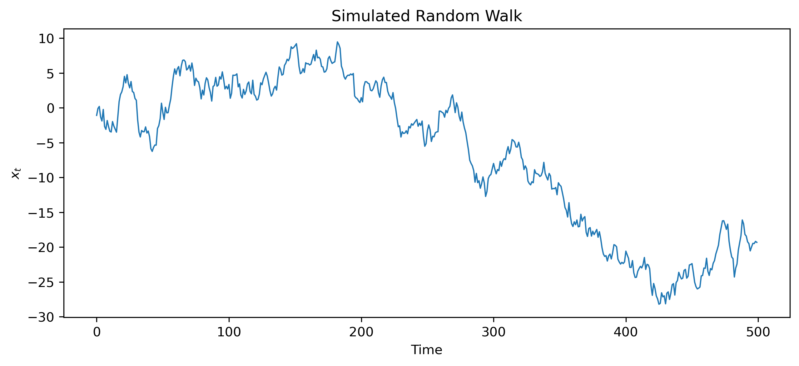

10.3 Why Random Walks Matter¶

Random walks are central in economics and finance.

Examples include:

stock prices
exchange rates
some macroeconomic aggregates

The random walk model implies:

strong persistence
unpredictable long-run movement
permanent effects of shocks

10.4 The Unit Root Idea¶

The random walk can be rewritten as:

x_t = \phi x_{t-1} + w_t

with:

\phi = 1

Big Picture

Unit root processes behave fundamentally differently from stationary processes:

shocks do not fade away
the series does not return to a stable level
variability grows over time

Nonstationary → Difference → Stationary → Model

10.5 Why the Unit Root Matters¶

Consider:

x_t = \phi x_{t-1} + w_t

(1)

Case 1: $|\phi| < 1$ ¶

shocks gradually disappear
the series returns toward a stable mean
the process is stationary

Case 2: $\phi = 1$ ¶

shocks never disappear
the series accumulates past shocks
the process becomes nonstationary

10.6 Stationary vs Unit Root Processes¶

Stationary Process¶

stable mean
stable variance
temporary shocks

Unit Root Process¶

drifting behavior
growing variance
permanent shocks

10.7 Simulating Different Levels of Persistence¶

np.random.seed(123)

n = 500
w = np.random.normal(0,1,n)

x1 = np.zeros(n)
x2 = np.zeros(n)
x3 = np.zeros(n)

phi1 = 0.4
phi2 = 0.9
phi3 = 1.0

for t in range(1,n):
    x1[t] = phi1*x1[t-1] + w[t]
    x2[t] = phi2*x2[t-1] + w[t]
    x3[t] = phi3*x3[t-1] + w[t]

fig, ax = plt.subplots(3,1, figsize=(10,8))

ax[0].plot(x1)
ax[0].set_title(r"$\phi = 0.4$")

ax[1].plot(x2)
ax[1].set_title(r"$\phi = 0.9$")

ax[2].plot(x3)
ax[2].set_title(r"$\phi = 1.0$ (Unit Root)")

plt.tight_layout()

plt.savefig("figs/ch10/ar-sim.png", dpi=300, bbox_inches="tight")
plt.close()   # replace with plt.show()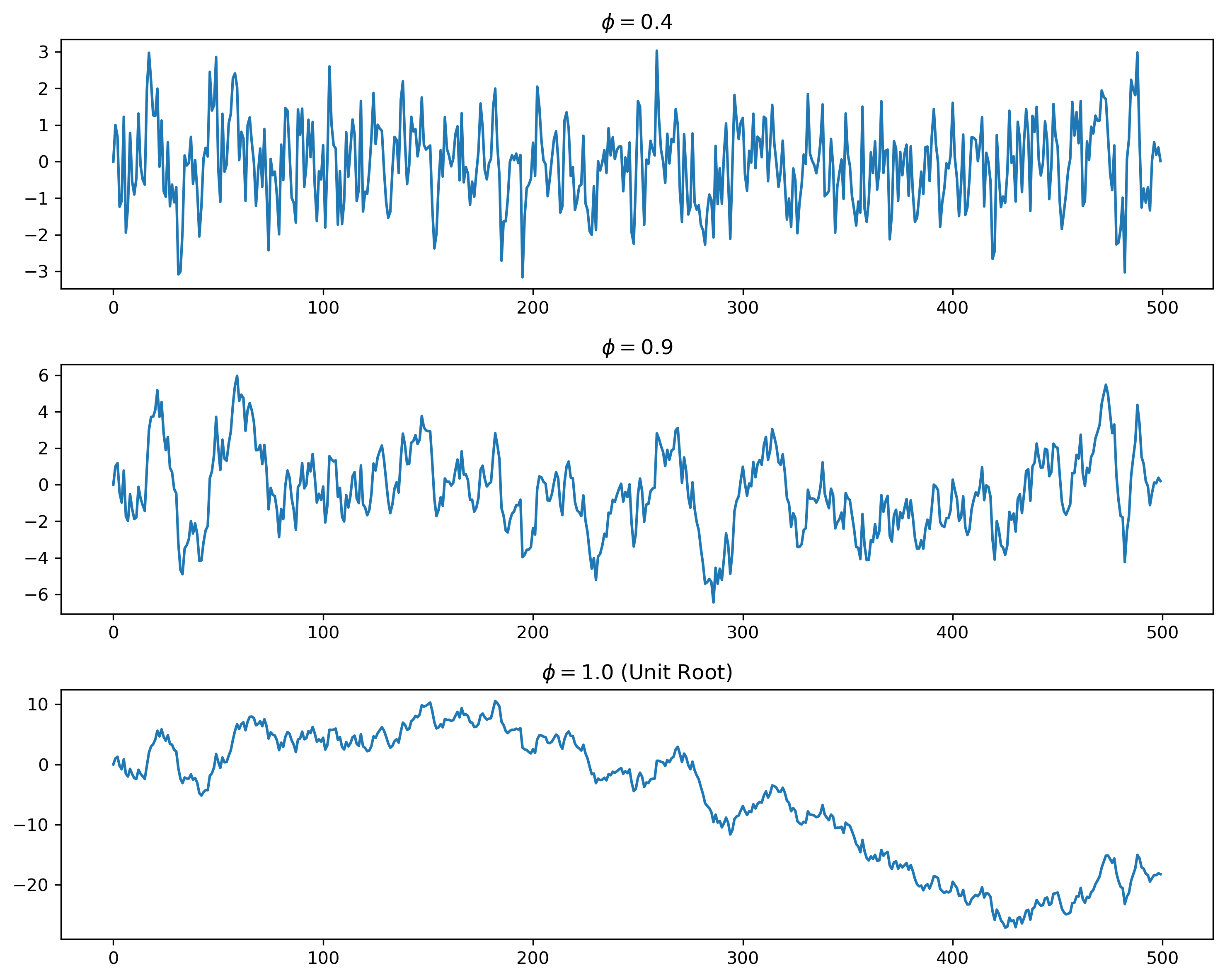

10.8 Differencing¶

A common way to remove unit roots is differencing.

10.9 Differencing a Random Walk¶

For a random walk:

x_t = x_{t-1} + w_t

Taking first differences:

\Delta x_t = x_t - x_{t-1} = w_t

10.10 Simulating Differencing¶

dx = np.diff(x)

plt.figure(figsize=(10,4))
plt.plot(dx, lw=1)
plt.title("First Difference of Random Walk")
plt.xlabel("Time")
plt.ylabel(r"$\Delta x_t$")

plt.savefig("figs/ch10/rw-diff.png", dpi=300, bbox_inches="tight")
plt.close()   # replace with plt.show()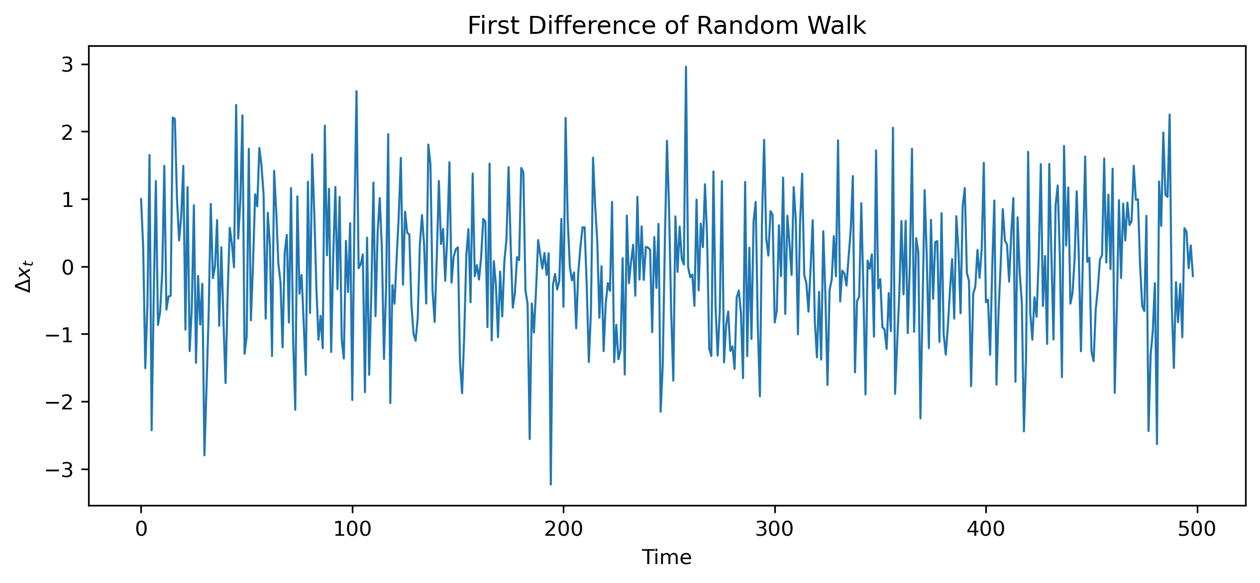

10.11 Integrated Processes¶

A unit root process is said to be integrated of order one.

Example¶

Series	Order
White noise	$I(0)$
Random walk	$I(1)$

10.12 Detrending vs Differencing¶

Nonstationarity may arise for different reasons.

Deterministic Trend¶

Suppose:

x_t = \alpha + \beta t + u_t

(3)

where $u_t$ is stationary.

Removing the trend may produce stationarity.

Stochastic Trend¶

For a random walk:

x_t = x_{t-1} + w_t

(4)

detrending alone is insufficient.

Differencing is required.

10.13 Visual Comparison¶

np.random.seed(123)

t = np.arange(500)

trend_stationary = 0.03*t + np.random.normal(0,1,500)

plt.figure(figsize=(10,4))
plt.plot(trend_stationary)
plt.title("Trend-Stationary Series")
plt.xlabel("Time")

plt.savefig("figs/ch10/trend.png", dpi=300, bbox_inches="tight")
plt.close()   # replace with plt.show()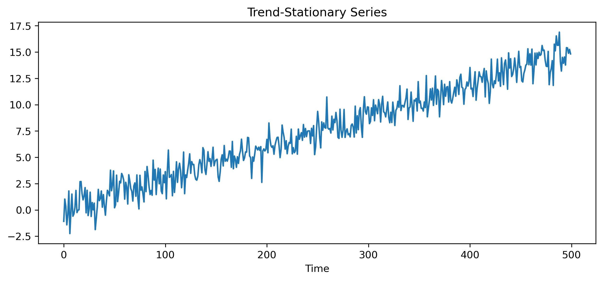

10.14 Why Unit Roots Matter¶

Unit roots affect:

forecasting
inference
regression
model selection

This problem becomes central later in:

spurious regression
cointegration
ECM models

10.15 The Dickey–Fuller Test¶

We now need a way to test for unit roots.

Consider:

x_t = \phi x_{t-1} + w_t

Subtract $x_{t-1}$ from both sides:

x_t - x_{t-1} = (\phi - 1)x_{t-1} + w_t

or:

\Delta x_t = \theta x_{t-1} + w_t

where:

\theta = \phi - 1

Hypotheses¶

H_0: \theta = 0 \quad \text{(unit root)}

H_1: \theta < 0 \quad \text{(stationary)}

10.16 Augmented Dickey–Fuller (ADF) Test¶

Real-world data often exhibit serial correlation.

The Augmented Dickey–Fuller (ADF) test extends the Dickey–Fuller test by including lagged differences:

\Delta x_t = \alpha + \theta x_{t-1} + \sum_{i=1}^p \gamma_i \Delta x_{t-i} + u_t

(5)

10.17 Interpreting the ADF Test¶

Reject $H_0$ ¶

evidence against a unit root
series likely stationary

Fail to Reject $H_0$ ¶

insufficient evidence against a unit root
series may be nonstationary

10.18 ADF Testing in Gretl¶

Variable → Unit root tests → Augmented Dickey-Fuller

Typical Steps¶

Choose variable
Include constant and/or trend if appropriate
Select lag length
Interpret test statistic and p-value

[GRETL Screenshot Placeholder: ADF test dialog]

[GRETL Screenshot Placeholder: ADF test output]

10.19 KPSS Test (Optional)¶

The KPSS test reverses the hypotheses.

KPSS Hypotheses¶

H_0: \text{stationary}

H_1: \text{unit root}

10.20 Looking Ahead¶

In this chapter, we introduced:

unit roots
differencing
ADF testing

We are now ready to build formal stochastic models for stationary time series.

In the next chapters, we study:

autoregressive (AR) models
moving average (MA) models
ARMA and ARIMA models

Key Takeaways¶

Concept Check¶

Basic¶

What is a unit root?
What does it mean for a time series to be nonstationary?
What is a random walk?

Intuition¶

Why do shocks have permanent effects in a unit root process?
Why does a random walk not return to a stable level?
Why is nonstationarity problematic for modeling?

Intermediate¶

What is the purpose of differencing a time series?
What is the difference between:
- a stationary process
- a unit root process
What is the difference between:
- deterministic trend
- stochastic trend

Finance Insight¶

Why are stock prices often modeled as random walks?
Why are returns typically stationary?

Challenge¶

Suppose a series becomes stationary after differencing once.

What does this imply about the original series?

Interpretation & Practice¶

A time series shows a strong upward trend and does not return to a stable level.
- What does this suggest?
- What might be an appropriate transformation?

A series appears to “wander” over time.
- What type of process might this be?
- What does this imply about shocks?

After differencing, a series fluctuates around zero.
- What does this suggest?
- Why is this useful?

A regression between two trending series shows a strong relationship.
- Why might this be misleading?
- What concept does this illustrate?

A series has a deterministic upward trend.
- Would differencing or detrending be more appropriate?
- Why?

Finance Interpretation¶

A stock price series is nonstationary.
- Why is modeling prices directly problematic?
- Why are returns preferred?

A return series appears stable over time.
- What does this suggest?
- Why is this important?

Challenge¶

Suppose you difference a stationary series.
- What might happen?
- Why is over-differencing a problem?

Numerical Practice¶

Random Walk and Differencing¶

Suppose a random walk is defined as:

x_t = x_{t-1} + w_t

with:

$x_0 = 100$
shocks: 2, −1, 3, −2

Compute $x_1, x_2, x_3, x_4$

Compute the first differences:

\Delta x_t = x_t - x_{t-1}

What do you observe?
What does this suggest?

Identifying Nonstationarity¶

Consider the series:
10, 12, 15, 19, 24

Does this appear stationary?
Compute the first differences
Does the differenced series look more stable?

Trend vs Difference¶

Suppose:

x_t = 5 + 0.5t + u_t

What type of trend is this?
Would differencing remove it?
What would the differenced series look like?

ADF Interpretation (Applied)¶

Consider the following output from an Augmented Dickey–Fuller (ADF) test:

Augmented Dickey-Fuller Test

Test Statistic:   -1.85
p-value:           0.67
Lags Used:         2
Observations:      197

Critical Values:
  1% level:       -3.46
  5% level:       -2.88
 10% level:       -2.57

What is the null hypothesis of the ADF test?
Compare the test statistic with the critical values.
- Is the test statistic more negative than the 5% critical value?
Based on the p-value and test statistic:
- Do you reject the null hypothesis?
- What does this imply about the series?
What would you do next before modeling this series?

Second Example¶

Now consider:

Augmented Dickey-Fuller Test

Test Statistic:   -3.25
p-value:           0.02
Lags Used:         1
Observations:      198

Critical Values:
  1% level:       -3.46
  5% level:       -2.88
 10% level:       -2.57

Do you reject the null hypothesis at the 5% level?
What does this imply about stationarity?
Why might the test statistic be compared with critical values rather than relying only on the p-value?

Challenge¶

Suppose the test statistic is close to the critical value.
- Why might conclusions be uncertain?
- What additional checks could you perform?

Suppose you difference a series twice.

When might this be necessary?
What is the risk of doing this unnecessarily?

Suppose two nonstationary series are regressed on each other.

Why might the results be misleading?
What concept does this relate to?

Chapter 10 — Unit Roots and Differencing

Learning Objectives¶

10.1 Persistence Revisited¶

10.2 Simulating a Random Walk¶

10.3 Why Random Walks Matter¶

10.4 The Unit Root Idea¶

10.5 Why the Unit Root Matters¶

Case 1: ∣ϕ∣<1|\phi| < 1∣ϕ∣<1¶

Case 2: ϕ=1\phi = 1ϕ=1¶

10.6 Stationary vs Unit Root Processes¶

Stationary Process¶

Unit Root Process¶

10.7 Simulating Different Levels of Persistence¶

10.8 Differencing¶

10.9 Differencing a Random Walk¶

10.10 Simulating Differencing¶

10.11 Integrated Processes¶

Example¶

10.12 Detrending vs Differencing¶

Deterministic Trend¶

Stochastic Trend¶

10.13 Visual Comparison¶

10.14 Why Unit Roots Matter¶

10.15 The Dickey–Fuller Test¶

Hypotheses¶

10.16 Augmented Dickey–Fuller (ADF) Test¶

10.17 Interpreting the ADF Test¶

Reject H0H_0H0​¶

Fail to Reject H0H_0H0​¶

10.18 ADF Testing in Gretl¶

Menu¶

Typical Steps¶

10.19 KPSS Test (Optional)¶

KPSS Hypotheses¶

10.20 Looking Ahead¶

Key Takeaways¶

Concept Check¶

Basic¶

Intuition¶

Intermediate¶

Finance Insight¶

Challenge¶

Interpretation & Practice¶

Finance Interpretation¶

Challenge¶

Numerical Practice¶

Random Walk and Differencing¶

Identifying Nonstationarity¶

Trend vs Difference¶

ADF Interpretation (Applied)¶

Second Example¶

Challenge¶

Case 1: $|\phi| < 1$ ¶

Case 2: $\phi = 1$ ¶

Reject $H_0$ ¶

Fail to Reject $H_0$ ¶