Chapter 17 — Spurious Regression
In earlier chapters, we learned that many time series are nonstationary. We also saw that random walks can drift over time even when they are generated only by random shocks.
We now study one of the most important warnings in applied time series regression:
This problem is especially common when working with nonstationary data, such as random walks or trending variables.
Learning Objectives
By the end of this chapter, you should be able to:
explain what spurious regression means
understand why nonstationary series can produce misleading regression results
recognize warning signs such as high and persistent residuals
use residual diagnostics to detect problems
understand why differencing may solve the problem
distinguish spurious regression from cointegration
17.1 The Basic Problem
Suppose we regress one time series on another:
In ordinary regression analysis, a statistically significant might suggest that is related to .
But with time series data, especially nonstationary data, this conclusion can be misleading.
This is the problem of spurious regression.
The model may report:
high
statistically significant coefficients
convincing-looking results
But these are driven by shared trending behavior — not by a true economic relationship.
17.2 Why Nonstationarity Creates Trouble
Consider two independent random walks:
and
where and are independent white noise processes.
By construction, there is no true relationship between and .
Yet both series may drift over time.
If two unrelated random walks drift in similar directions over a sample period, a regression may interpret that common movement as evidence of a relationship.
17.3 Symptoms of Spurious Regression
A spurious regression often produces:
high
significant t-statistics
low Durbin–Watson statistic
persistent residuals
residual autocorrelation
This is one reason why time series regression requires additional diagnostic checks.
17.4 A Simple Simulation
Let us simulate two independent random walks.
import numpy as np
import matplotlib.pyplot as plt

np.random.seed(124)

n = 200

u = np.random.standard_normal(n)
v = np.random.standard_normal(n)

x = np.cumsum(u)
y = np.cumsum(v)

plt.figure(figsize=(10, 5))
plt.plot(x, label="x")
plt.plot(y, label="y")
plt.title("Two Independent Random Walks")
plt.xlabel("Time")
plt.ylabel("Value")
plt.legend()

plt.savefig("figs/ch17/rw.png", dpi=300, bbox_inches="tight")
plt.close()   # replace with plt.show()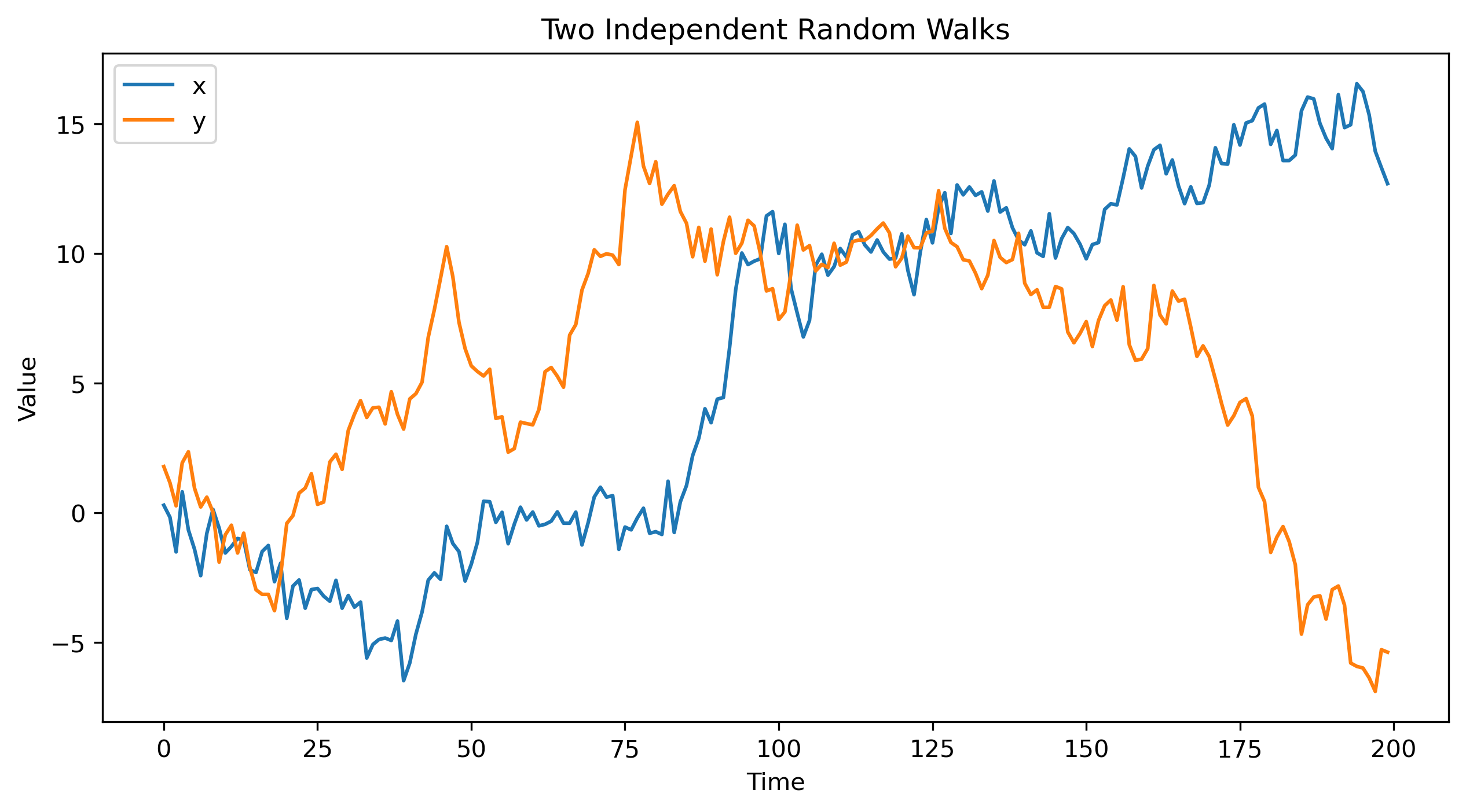
17.5 Regressing One Random Walk on Another
Now regress on :
import statsmodels.api as sm

X = sm.add_constant(x)
model = sm.OLS(y, X)
results = model.fit()

print(results.summary())
OLS Regression Results
==============================================================================
Dep. Variable: y R-squared: 0.001
Model: OLS Adj. R-squared: -0.004
Method: Least Squares F-statistic: 0.2312
Date: Wed, 29 Apr 2026 Prob (F-statistic): 0.631
Time: 14:10:42 Log-Likelihood: -607.38
No. Observations: 200 AIC: 1219.
Df Residuals: 198 BIC: 1225.
Df Model: 1
Covariance Type: nonrobust
==============================================================================
coef std err t P>|t| [0.025 0.975]
------------------------------------------------------------------------------
const 5.4880 0.469 11.692 0.000 4.562 6.414
x1 0.0249 0.052 0.481 0.631 -0.077 0.127
==============================================================================
Omnibus: 15.351 Durbin-Watson: 0.038
Prob(Omnibus): 0.000 Jarque-Bera (JB): 16.030
Skew: -0.654 Prob(JB): 0.000330
Kurtosis: 2.538 Cond. No. 12.0
==============================================================================
Notes:
[1] Standard Errors assume that the covariance matrix of the errors is correctly specified.The output will often show a statistically significant coefficient, even though the two variables were generated independently.
This is the essence of spurious regression.
17.6 Why This Is Problematic
Both and are nonstationary random walks.
Standard regression inference relies on assumptions that are violated in this setting.
This can lead to:
misleading t-statistics
invalid p-values
false confidence in the estimated relationship
17.7 Residual Diagnostics
A key diagnostic is to examine the residuals.
If a regression relationship is meaningful, the residuals should be stationary.
If the residuals remain nonstationary, the regression has not captured a stable relationship.
Residual Plot
uhat = results.resid

plt.figure(figsize=(10, 4))
plt.plot(uhat, linewidth=1.5)
plt.axhline(0, color="black", linestyle="--", linewidth=1)
plt.title("Residuals from Spurious Regression")
plt.xlabel("Time")
plt.ylabel("Residual")

plt.savefig("figs/ch17/res.png", dpi=300, bbox_inches="tight")
plt.close()   # replace with plt.show()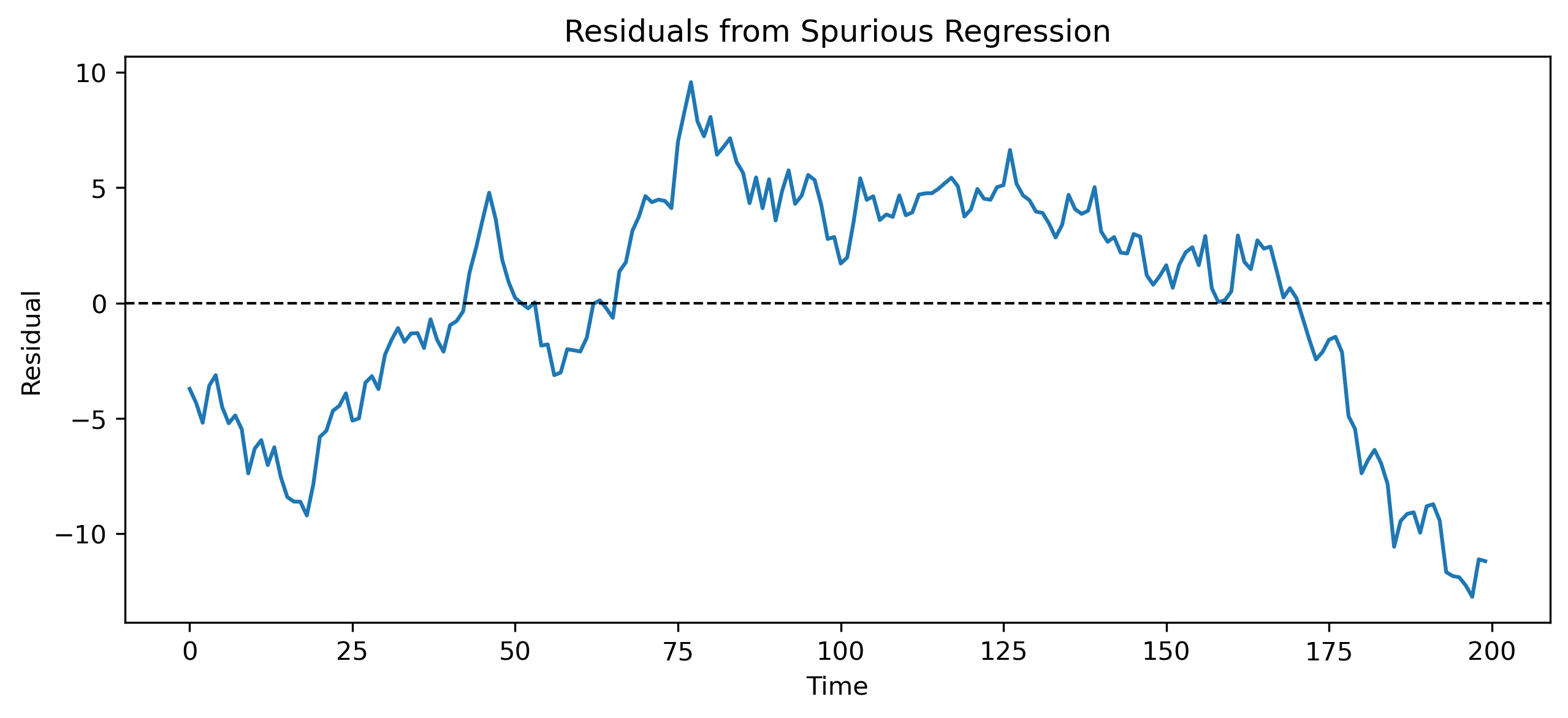
Residual ACF
from statsmodels.graphics.tsaplots import plot_acf

plot_acf(uhat, lags=40)
plt.title("ACF of Residuals")

plt.savefig("figs/ch17/res_acf.png", dpi=300, bbox_inches="tight")
plt.close()   # replace with plt.show()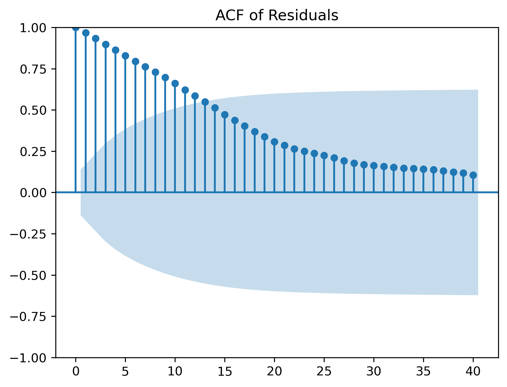
17.8 Unit Root Testing
To formally check nonstationarity, we can perform unit root tests.
For the original series, we expect:
to be nonstationary
to be nonstationary
For a spurious regression, residuals are often nonstationary as well.
from statsmodels.tsa.stattools import adfuller

def adf_summary(series, name):
    result = adfuller(series)
    print(f"ADF test for {name}")
    print(f"ADF statistic: {result[0]:.4f}")
    print(f"p-value: {result[1]:.4f}")
    print("Critical values:")
    for key, value in result[4].items():
        print(f"  {key}: {value:.4f}")
    print()

adf_summary(x, "x")
adf_summary(y, "y")
adf_summary(uhat, "residuals")
ADF test for x
ADF statistic: -0.7378
p-value: 0.8367
Critical values:
1%: -3.4638
5%: -2.8763
10%: -2.5746
ADF test for y
ADF statistic: -0.6210
p-value: 0.8662
Critical values:
1%: -3.4636
5%: -2.8762
10%: -2.5746
ADF test for residuals
ADF statistic: -0.5837
p-value: 0.8746
Critical values:
1%: -3.4636
5%: -2.8762
10%: -2.574617.9 Fixing the Problem: Differencing
A common solution is to difference the data.
Instead of estimating:
we estimate:
where:
and:
Regression in Differences
d_x = np.diff(x)
d_y = np.diff(y)

D_X = sm.add_constant(d_x)

diff_model = sm.OLS(d_y, D_X)
diff_results = diff_model.fit()

print(diff_results.summary())
OLS Regression Results
==============================================================================
Dep. Variable: y R-squared: 0.005
Model: OLS Adj. R-squared: -0.000
Method: Least Squares F-statistic: 0.9755
Date: Wed, 29 Apr 2026 Prob (F-statistic): 0.325
Time: 14:14:36 Log-Likelihood: -279.21
No. Observations: 199 AIC: 562.4
Df Residuals: 197 BIC: 569.0
Df Model: 1
Covariance Type: nonrobust
==============================================================================
coef std err t P>|t| [0.025 0.975]
------------------------------------------------------------------------------
const -0.0405 0.070 -0.576 0.565 -0.179 0.098
x1 0.0719 0.073 0.988 0.325 -0.072 0.215
==============================================================================
Omnibus: 0.339 Durbin-Watson: 1.967
Prob(Omnibus): 0.844 Jarque-Bera (JB): 0.181
Skew: -0.067 Prob(JB): 0.914
Kurtosis: 3.063 Cond. No. 1.08
==============================================================================
Notes:
[1] Standard Errors assume that the covariance matrix of the errors is correctly specified.This is what we should expect, because the two random walks were generated from independent shocks.
17.10 Interpretation
Spurious regression arises because nonstationary series can move together over time even when there is no true relationship.
Differencing often solves the problem by removing the stochastic trend.
However, differencing is not always the final answer.
Sometimes nonstationary variables really do move together because of a long-run equilibrium relationship.
This leads to the idea of cointegration.
17.11 Connection to Cointegration
There is one important exception to the warning about regressions in levels.
In other words:
nonstationary residuals → spurious regression
stationary residuals → possible cointegration
We return to this idea in Chapter 20.
17.12 GRETL Example
We now reproduce the simulation and regression in GRETL.
Step 1: Create Data in GRETL
Menu
Set up for data entry:
File → New data setSelect:
Time series: T = 200Choose frequency:
Other
This creates an index variable.
Then generate two white-noise variables:
Add → Random variable → Normal distribution
Generate:
uv
Then create cumulative sums:
Add → Define new variable
Use:
x = cum(u)
y = cum(v)
Command
nulldata 200
set seed 124

series u = normal()
series v = normal()

series x = cum(u)
series y = cum(v)
Step 2: Plot the Series
Menu
Graph → Time series plot
Select:
xy
Command
gnuplot x y --time-series --with-lines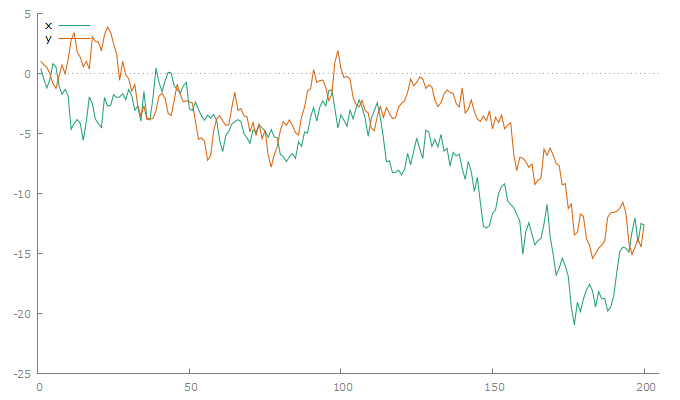
Figure 1:Two independent random walks
Step 3: Run the Spurious Regression
Menu
Model → Ordinary Least Squares
Dependent variable:
yIndependent variable:
x
Command
ols y const xExample output:
Model 1: OLS, using observations 1-200
Dependent variable: y

             coefficient   std. error   t-ratio    p-value
  ---------------------------------------------------------
  const       0.578591     0.295706      1.957    0.0518    *
  x           0.660102     0.0333565    19.79     8.40e-049 ***

Mean dependent var  −4.061555   S.D. dependent var   4.385945
Sum squared resid    1285.510   S.E. of regression   2.548033
R-squared            0.664188   Adjusted R-squared   0.662492
F(1, 198)            391.6158   P-value(F)           8.40e-49
Log-likelihood      −469.8470   Akaike criterion     943.6941
Schwarz criterion 950.2907 Hannan-Quinn 946.3636Step 4: Save and Plot Residuals
Menu
In the regression window:
Save → Residuals
Command
series uhat = $uhat
gnuplot uhat --time-series --with-lines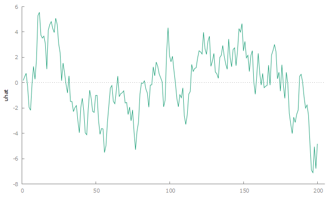
Figure 2:Residuals from the spurious regression
The residuals still show persistent behavior.
Step 5: Check Residual Autocorrelation
Menu
Variable → Correlogram
Select uhat.
If you do not see this option, go to:
Data → Dataset structure...
and select:
Time series → Other
You can also right click on uhat and select Correlogram.
Command
corrgm uhat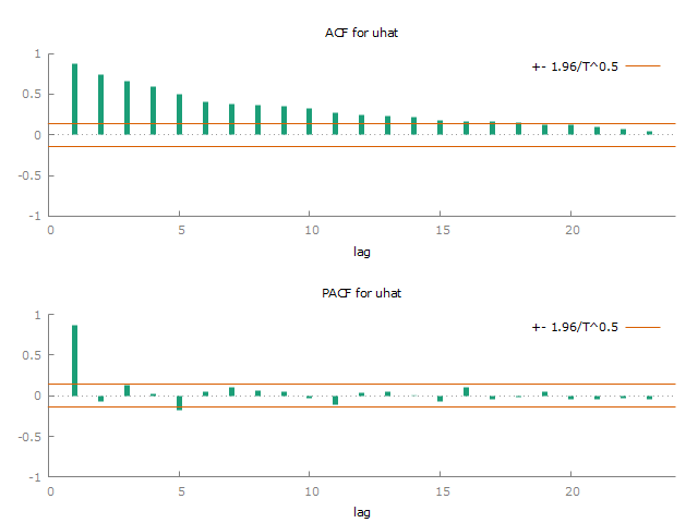
Figure 3:Correlogram of residuals
Step 6: ADF Tests
Menu
Variable → Unit root tests → Augmented Dickey-Fuller
Test:
xyuhat
Command
adf 0 x
adf 0 y
adf 0 uhat
It is often better to use the menu because GRETL can help determine an appropriate lag length for the ADF test.
Example output for x:
Augmented Dickey-Fuller test for x
testing down from 14 lags, criterion AIC
sample size 199
unit-root null hypothesis: a = 1

  test with constant
  including 0 lags of (1-L)x
  model: (1-L)y = b0 + (a-1)*y(-1) + e
  estimated value of (a - 1): -0.0224933
  test statistic: tau_c(1) = -1.57309
  asymptotic p-value 0.4964
Example output for y:
Augmented Dickey-Fuller test for y
testing down from 14 lags, criterion AIC
sample size 199
unit-root null hypothesis: a = 1

  test with constant
  including 0 lags of (1-L)y
  estimated value of (a - 1): -0.0198401
  test statistic: tau_c(1) = -1.22352
  asymptotic p-value 0.6666
Example output for uhat:
Augmented Dickey-Fuller test for uhat
testing down from 14 lags, criterion AIC
sample size 195
unit-root null hypothesis: a = 1

  test with constant
  including 4 lags of (1-L)uhat
  estimated value of (a - 1): -0.117113
  test statistic: tau_c(1) = -2.93493
asymptotic p-value 0.04143Step 7: Difference the Data
Menu
Select x and y, right click, and choose:
Add differences
Command
series d_x = diff(x)
series d_y = diff(y)
Step 8: Re-estimate the Regression in Differences
Menu
Model → Ordinary Least Squares
Dependent variable:
d_yIndependent variable:
d_x
Command
ols d_y const d_xExample output:
Model 2: OLS, using observations 2-200 (T = 199)
Dependent variable: d_y

             coefficient   std. error   t-ratio   p-value
  -------------------------------------------------------
  const      −0.0721970    0.0706927    −1.021    0.3084
  d_x        −0.0574247    0.0647031    −0.8875   0.3759

Mean dependent var  −0.068429   S.D. dependent var   0.994910
Sum squared resid    195.2089   S.E. of regression   0.995444
R-squared            0.003982   Adjusted R-squared  -0.001073
F(1, 197)            0.787676   P-value(F)           0.375886
Log-likelihood      −280.4549   Akaike criterion     564.9099
Schwarz criterion    571.4965   Hannan-Quinn         567.5757
rho 0.000807 Durbin-Watson 1.97873217.13 Practical Checklist
17.14 Common Mistakes
17.15 Looking Ahead
Spurious regression teaches us a central lesson:
In the next chapter, we introduce dynamic regression models, including distributed lag models and ARDL models.
These models allow us to study how variables affect each other over time.
Key Takeaways
Concept Check
Basic
What is spurious regression?
Why can two unrelated time series appear to be related?
What role does nonstationarity play in spurious regression?
Intuition
Why do random walks tend to drift over time?
How can two independent random walks appear to move together?
Why is a high not reliable evidence of a relationship in time series data?
Intermediate
What assumptions of classical regression are violated with nonstationary data?
Why are t-statistics and p-values unreliable in spurious regressions?
What is the key diagnostic principle involving residuals?
Diagnostics
What does it mean if regression residuals are nonstationary?
Why is residual autocorrelation a warning sign?
Fixing the Problem
Why does differencing often remove spurious relationships?
Challenge
Can a regression in levels ever be valid with nonstationary variables?
Explain.
Interpretation & Practice
A regression produces:
high
significant coefficient
strong trend in residuals
What does this suggest?
Two variables trend upward over time.
Regression shows strong relationship.
What is the key concern?
Residuals from a regression appear highly persistent.
What does this imply?
After differencing, the regression coefficient becomes insignificant.
What does this suggest about the original relationship?
ADF test fails to reject unit root for residuals.
What does this imply?
Suppose inflation and GDP both trend upward.
Regression suggests a strong relationship.
What must you check before concluding causality?
Challenge
A regression in levels produces stationary residuals.
What does this suggest?
What concept does this relate to?
Numerical Practice
Random Walk Construction
Suppose:
with shocks:
and .
Compute
Differencing
Using the values above:
Compute
Interpretation
Why is stationary but is not?
Regression Output
Suppose a regression produces:
coefficient significant
residuals highly autocorrelated
What is the likely problem?
ADF Interpretation
Suppose you estimate a regression between two time series and obtain the following ADF test results:
| Series | ADF p-value |
|---|---|
| 0.82 | |
| 0.76 | |
| residuals | 0.80 |
What do these results suggest about and ?
Are the residuals stationary?
Is the regression likely to be spurious?
Now consider an alternative case:
| Series | ADF p-value |
|---|---|
| 0.88 | |
| 0.91 | |
| residuals | 0.02 |
What do these results suggest about and ?
Are the residuals stationary?
What does this imply about the regression?
What concept does this relate to?
Why is it possible for and to be nonstationary, but the residuals to be stationary?
Model Comparison
Suppose:
Levels regression shows strong relationship
Differences regression shows no relationship
What conclusion should you draw?
Challenge
Suppose you regress two random walks and obtain:
significant coefficient
high
Why is this misleading?
What underlying property causes this?
Suppose residuals are stationary.
What does this imply?
What is the next step in analysis?
Appendix 17A — Why Nonstationarity Leads to Spurious Regression
This appendix provides an intuitive but slightly more formal explanation of why regressions involving nonstationary time series can produce misleading results.
A.1 Setup
Consider two independent random walks:
Assume:
and are independent
there is no true relationship between and
A.2 Accumulation of Shocks
A random walk can be written as:
so its variance is:
This is the defining feature of nonstationarity.
A.3 Persistent Trending Behavior
Because shocks accumulate:
both and tend to drift over time
they exhibit persistent trending behavior
Even though these trends are random, they can look systematic in finite samples.
A.4 The Regression Problem
Now consider the regression:
The OLS estimator is:
This expression is written in simplified mean-zero form. The same intuition applies when an intercept is included.
A.5 Why the Estimator Misbehaves
Even though and are independent:
both contain persistent trends
large values of may coincide with large values of
both and can grow because shocks accumulate
A.6 Failure of Standard Inference
Standard regression theory assumes:
constant variance
weak dependence
stable distributions over time
But with nonstationary data:
variance increases with time
shocks have long-lasting effects
observations are highly dependent
A.7 Residual Behavior
If the regression were meaningful, the residuals should be stationary.
However:
often inherits nonstationarity from and .
A.8 Big Picture
A.9 How to Fix the Problem
There are two main approaches:
difference the data, focusing on short-run relationships
test for cointegration, recovering possible long-run relationships