Chapter 15 — Forecasting Methods

So far, we have studied how time series behave and how they can be modeled using AR, MA, ARMA, and ARIMA models.

We now turn to one of the main practical goals of time series analysis:

Forecasting is important in economics, business, finance, and policy.

Examples include:

forecasting inflation
predicting GDP growth
projecting demand
forecasting exchange rates
estimating future sales
predicting stock volatility

This chapter introduces the basic logic of forecasting.

Learning Objectives¶

By the end of this chapter, you should be able to:

explain what a forecast is
distinguish in-sample fit from out-of-sample forecasting
distinguish one-step-ahead and multi-step-ahead forecasts
understand static and dynamic forecasts
generate forecasts from simple time series models
interpret forecast uncertainty
understand the basic forecasting workflow

15.1 What Is a Forecast?¶

A forecast is a prediction of a future value based on information available today.

Suppose we observe:

x_1, x_2, \dots, x_T

A forecast of $x_{T+1}$ is written as:

\hat{x}_{T+1}

More generally, an $h$ -step-ahead forecast is:

\hat{x}_{T+h}

15.2 Forecasting Is Conditional¶

Forecasting is always based on available information.

At time $T$ , we know:

x_1, x_2, \dots, x_T

but we do not yet know:

x_{T+1}, x_{T+2}, \dots

A forecast is therefore conditional on the information set available at time $T$ .

15.3 Forecast vs Fitted Value¶

It is important to distinguish a forecast from a fitted value.

A fitted value is produced for an observation already in the sample.

A forecast is produced for an observation not yet observed.

Concept	Meaning
fitted value	model prediction for an observed data point
forecast	model prediction for a future data point

This is why out-of-sample evaluation is essential.

15.4 In-Sample vs Out-of-Sample Forecasting¶

In-Sample Fit¶

In-sample fit refers to how well the model explains data already used for estimation.

For example, if we estimate a model using observations 1 to $T$ , then fitted values within this same range are in-sample.

Out-of-Sample Forecasting¶

Out-of-sample forecasting evaluates how well the model predicts observations not used in estimation.

15.5 Train-Test Split for Time Series¶

In cross-sectional data, observations are often randomly split into training and testing samples.

In time series, we do not randomly shuffle observations.

Instead, we preserve time order.

For example:

estimate model using observations $1,\dots,T_0$
forecast observations $T_0+1,\dots,T$
compare forecasts with actual values

15.6 One-Step-Ahead Forecasts¶

A one-step-ahead forecast predicts the next observation.

At time $T$ , the one-step-ahead forecast is:

\hat{x}_{T+1}

For an AR(1) model:

x_t = \phi x_{t-1} + w_t

the one-step-ahead forecast is:

\hat{x}_{T+1} = \phi x_T

because the best prediction of the future shock is zero:

E[w_{T+1}] = 0

15.7 Multi-Step-Ahead Forecasts¶

A multi-step-ahead forecast predicts more than one period into the future.

For AR(1):

x_t = \phi x_{t-1} + w_t

the two-step-ahead forecast is:

\hat{x}_{T+2} = \phi \hat{x}_{T+1} = \phi^2 x_T

More generally:

\hat{x}_{T+h} = \phi^h x_T

If the mean is not zero, forecasts return toward:

\frac{\mu}{1-\phi}

15.8 Forecasting a Random Walk¶

For a random walk:

x_t = x_{t-1} + w_t

the best forecast of tomorrow is today’s value:

\hat{x}_{T+1} = x_T

For any horizon $h$ :

\hat{x}_{T+h} = x_T

15.9 Forecasting a Random Walk with Drift¶

For a random walk with drift:

x_t = \delta + x_{t-1} + w_t

the $h$ -step-ahead forecast is:

\hat{x}_{T+h} = x_T + h\delta

15.10 Static vs Dynamic Forecasts¶

Forecasting software often distinguishes between static and dynamic forecasts.

Static Forecasts¶

A static forecast uses actual lagged values whenever they are available.

For example, in an AR(1):

\hat{x}_{t} = \hat{\phi}x_{t-1}

uses the actual value $x_{t-1}$ .

Dynamic Forecasts¶

A dynamic forecast uses previous forecasts as inputs when actual future values are unavailable.

For example:

\hat{x}_{t} = \hat{\phi}\hat{x}_{t-1}

15.11 Why Dynamic Forecasts Become Harder¶

Dynamic forecasts become less reliable as the horizon increases.

Why?

Because forecast errors accumulate.

This is especially important for:

macroeconomic forecasts
financial forecasts
demand forecasts
policy projections

15.12 Forecast Errors¶

A forecast error is the difference between the actual value and the forecast:

e_{T+h} = x_{T+h} - \hat{x}_{T+h}

A good forecast has small errors on average.

Forecast evaluation is the focus of the next chapter.

15.13 Forecast Intervals¶

A point forecast gives a single predicted value.

But forecasts are uncertain.

A forecast interval gives a range of plausible future values.

For example, instead of saying:

Inflation next year will be 3%.

we might say:

Inflation is forecast to be 3%, with a plausible range from 2% to 4%.

15.14 Simulating Forecasts from an AR(1)¶

import numpy as np
import matplotlib.pyplot as plt

np.random.seed(123)

n = 120
phi = 0.8
w = np.random.normal(size=n)

x = np.zeros(n)

for t in range(1, n):
    x[t] = phi*x[t-1] + w[t]

T = 100
h = 20

history = x[:T+1]

forecast = np.zeros(h)
forecast[0] = phi * history[-1]

for i in range(1, h):
    forecast[i] = phi * forecast[i-1]

forecast_index = np.arange(T+1, T+h+1)

plt.figure(figsize=(10,4))
plt.plot(np.arange(T+1), history, label="Observed")
plt.plot(forecast_index, forecast, linestyle="--", label="Forecast")
plt.axvline(T, linestyle=":", color="black")
plt.title("Dynamic Forecast from an AR(1) Model")
plt.xlabel("Time")
plt.ylabel("$x_t$")
plt.legend()

plt.savefig("figs/ch15/AR1_forecast.png", dpi=300, bbox_inches="tight")
plt.close()   # replace with plt.show()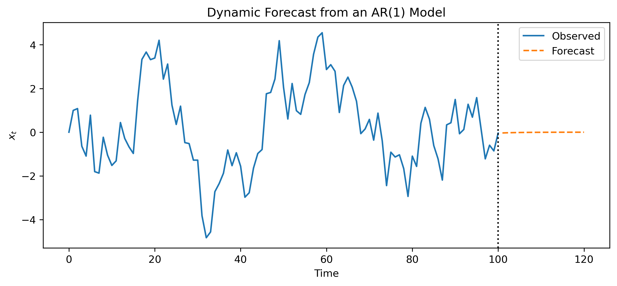

15.15 Forecasting Workflow¶

A practical forecasting workflow is:

plot the data
check stationarity
choose candidate models
estimate models
generate forecasts
compare forecasts with actual values
evaluate forecast errors
revise the model if needed

15.16 Gretl Example: Forecasting with ARIMA¶

We now outline a simple forecasting workflow in GRETL.

Step 1: Estimate a Model¶

Model → Time series → ARIMA

Choose:

dependent variable
AR order
differencing order
MA order

[GRETL Screenshot Placeholder: ARIMA model specification]

Step 2: Generate Forecasts¶

After estimating the model, in the model window:

Analysis → Forecasts

or:

Model window → Forecasts

depending on your GRETL version.

[GRETL Screenshot Placeholder: Forecast dialog]

Step 3: Choose Forecast Range¶

Choose:

forecast start date
forecast end date
static or dynamic forecast
whether to include forecast intervals

[GRETL Screenshot Placeholder: Forecast range and options]

Step 4: Inspect Forecast Output¶

GRETL typically provides:

forecast values
standard errors
confidence intervals
forecast graph

[GRETL Screenshot Placeholder: Forecast graph]

15.17 Common Mistakes¶

15.18 Looking Ahead¶

This chapter introduced the basic logic of forecasting.

In the next chapter, we study how to evaluate forecast accuracy.

We will examine:

bias
MSE
RMSE
MAE
MAPE
Theil’s U1 and U2
Decomposition

Key Takeaways¶

Concept Check¶

Basic¶

What is a forecast?
What does it mean for a forecast to be conditional?
What is the difference between a fitted value and a forecast?

Intuition¶

Why is forecasting fundamentally uncertain?
Why might a model fit past data well but perform poorly in forecasting?
Why is out-of-sample evaluation important?

Intermediate¶

What is the difference between:
- one-step-ahead forecasts
- multi-step-ahead forecasts
What is the difference between:
- static forecasts
- dynamic forecasts
Why do forecast errors tend to increase as the horizon grows?

Model-Based Forecasting¶

In an AR(1) model, why is the expected value of the future shock set to zero?
Why do AR(1) forecasts converge toward the long-run mean?

Challenge¶

Suppose a model produces very stable forecasts.

Does this necessarily mean it is accurate?

Interpretation & Practice¶

A model fits historical data extremely well but performs poorly out-of-sample.
- What might be the issue?
- What does this suggest about model evaluation?
A forecast for a stationary AR(1) process gradually flattens over time.
- Why does this happen?
A random walk forecast remains constant over time.
- What does this imply about predictability?
A forecast diverges rapidly as the horizon increases.
- What might this indicate about the underlying model?
Dynamic forecasts differ significantly from static forecasts.
- Why might this happen?

Finance Interpretation¶

A stock price follows a random walk.
- Why is the best forecast of tomorrow’s price today’s price?
A macroeconomic forecast becomes less precise over longer horizons.
- Why is this expected?

Challenge¶

A model produces very narrow forecast intervals.
- Why might this be misleading?
- What could be wrong with the model?

Numerical Practice¶

One-Step Forecast¶

Suppose:

x_t = 0.8 x_{t-1} + w_t

and $x_T = 10$ .

Compute the one-step-ahead forecast $\hat{x}_{T+1}$ .

Multi-Step Forecast¶

Using the same model:

Compute $\hat{x}_{T+2}$
Compute $\hat{x}_{T+3}$
What pattern do you observe?

Random Walk¶

Suppose:

x_t = x_{t-1} + w_t

and $x_T = 50$ .

Compute $\hat{x}_{T+1}$
Compute $\hat{x}_{T+5}$
What do you observe?

Random Walk with Drift¶

Suppose:

x_t = x_{t-1} + 2 + w_t

and $x_T = 100$ .

Compute $\hat{x}_{T+1}$
Compute $\hat{x}_{T+3}$

Forecast Error¶

Suppose:

forecast: $\hat{x}_{T+1} = 20$
actual: $x_{T+1} = 23$
Compute the forecast error.

Interpretation¶

Suppose forecast errors are consistently positive.

What does this imply about the model?

Dynamic Forecasting¶

Suppose a dynamic forecast is used.

Why might errors accumulate over time?

Challenge¶

Suppose two models produce:

Model A: very accurate one-step forecasts
Model B: better long-horizon forecasts
Which would you choose? Why?

You are forecasting monthly sales.

You estimate an AR(1) model and generate forecasts for the next 12 months.

Why might the 1-month-ahead forecast be reliable?
Why might the 12-month-ahead forecast be much less reliable?

Chapter 15 — Forecasting Methods

Learning Objectives¶

15.1 What Is a Forecast?¶

15.2 Forecasting Is Conditional¶

15.3 Forecast vs Fitted Value¶

15.4 In-Sample vs Out-of-Sample Forecasting¶

In-Sample Fit¶

Out-of-Sample Forecasting¶

15.5 Train-Test Split for Time Series¶

15.6 One-Step-Ahead Forecasts¶

15.7 Multi-Step-Ahead Forecasts¶

15.8 Forecasting a Random Walk¶

15.9 Forecasting a Random Walk with Drift¶

15.10 Static vs Dynamic Forecasts¶

Static Forecasts¶

Dynamic Forecasts¶

15.11 Why Dynamic Forecasts Become Harder¶

15.12 Forecast Errors¶

15.13 Forecast Intervals¶

15.14 Simulating Forecasts from an AR(1)¶

15.15 Forecasting Workflow¶

15.16 Gretl Example: Forecasting with ARIMA¶

Step 1: Estimate a Model¶

Menu¶

Step 2: Generate Forecasts¶

Step 3: Choose Forecast Range¶

Step 4: Inspect Forecast Output¶

15.17 Common Mistakes¶

15.18 Looking Ahead¶

Key Takeaways¶

Concept Check¶

Basic¶

Intuition¶

Intermediate¶

Model-Based Forecasting¶

Challenge¶

Interpretation & Practice¶

Finance Interpretation¶

Challenge¶

Numerical Practice¶

One-Step Forecast¶

Multi-Step Forecast¶

Random Walk¶

Random Walk with Drift¶

Forecast Error¶

Interpretation¶

Dynamic Forecasting¶

Challenge¶