Chapter 6 — Trading Indicators as Filters

In the previous chapter, we studied smoothing methods designed to reduce noise and reveal underlying structure.

Many popular trading indicators are built on exactly the same idea.

They attempt to:

smooth noisy price movements,
detect trends,
identify momentum,
and generate trading signals.

This chapter introduces several widely used technical indicators:

moving average crossover systems,
MACD,
RSI,
Bollinger Bands.

The emphasis is practical and intuition-first.

We interpret these indicators not as mysterious trading formulas, but as statistical filtering tools.

Learning Objectives¶

By the end of this chapter, you should be able to:

explain the intuition behind major trading indicators
understand moving average crossover systems
interpret MACD and momentum indicators
understand RSI and overbought/oversold signals
interpret Bollinger Bands
understand indicators as filters
implement indicators using Python
recognize limitations of technical indicators

6.1 Why Trading Indicators Exist¶

Financial prices contain substantial noise.

Daily fluctuations may reflect:

news,
speculation,
temporary sentiment,
random variation.

Traders therefore attempt to extract useful signals from noisy data.

Most indicators attempt to identify:

trends,
momentum,
reversals,
or unusual volatility.

6.2 Trend Following vs Mean Reversion¶

Many trading indicators implicitly rely on one of two ideas.

Trend Following¶

Prices that rise may continue rising.

Prices that fall may continue falling.

Examples:

moving average crossover systems,
MACD,
momentum strategies.

Mean Reversion¶

Prices that move too far away from normal levels may eventually reverse.

Examples:

RSI,
Bollinger Bands,
contrarian strategies.

6.3 Moving Averages Revisited¶

Recall from the previous chapter that moving averages smooth noisy fluctuations.

For trading applications, moving averages are often interpreted dynamically.

Traders compare:

short-run averages,
and long-run averages.

6.4 Moving Average Crossover Systems¶

One of the simplest trading systems uses two moving averages:

a short-run moving average,
and a long-run moving average.

Basic Logic¶

Bullish Signal¶

If the short moving average rises above the long moving average:

Buy signal

Bearish Signal¶

If the short moving average falls below the long moving average:

Sell signal

6.5 Example: Moving Average Crossover vs. MACD¶

import pandas as pd
import numpy as np
import matplotlib.pyplot as plt

# --- Generate synthetic price data ---
np.random.seed(42)

dates = pd.date_range(start="2024-01-01", periods=200)

prices = np.cumsum(np.random.randn(200)) + 100

df = pd.DataFrame(
    {"Close": prices},
    index=dates
)

# --- Moving Averages ---
df["MA12"] = df["Close"].rolling(window=12).mean()

df["MA26"] = df["Close"].rolling(window=26).mean()

# --- Trading Signals ---
df["Signal"] = np.where(
    df["MA12"] > df["MA26"],
    1,
    -1
)

df["Crossover"] = df["Signal"].diff()

# --- MACD Calculation ---
df["EMA12"] = df["Close"].ewm(
    span=12,
    adjust=False
).mean()

df["EMA26"] = df["Close"].ewm(
    span=26,
    adjust=False
).mean()

df["MACD"] = df["EMA12"] - df["EMA26"]

df["SignalLine"] = df["MACD"].ewm(
    span=9,
    adjust=False
).mean()

df["Histogram"] = (
    df["MACD"] - df["SignalLine"]
)

# --- Plot Figure ---
plt.figure(figsize=(12,8))

# ==================================================
# Top Panel: Prices and Moving Averages
# ==================================================

plt.subplot(2,1,1)

plt.plot(
    df.index,
    df["Close"],
    label="Close Price",
    color="black",
    alpha=0.7
)

plt.plot(
    df.index,
    df["MA12"],
    label="MA12",
    linewidth=2
)

plt.plot(
    df.index,
    df["MA26"],
    label="MA26",
    linewidth=2
)

# Buy Signals
buy = df[df["Crossover"] == 2]

plt.scatter(
    buy.index,
    buy["Close"],
    marker="^",
    s=100,
    label="Buy Signal"
)

# Sell Signals
sell = df[df["Crossover"] == -2]

plt.scatter(
    sell.index,
    sell["Close"],
    marker="v",
    s=100,
    label="Sell Signal"
)

plt.title("Moving Average Crossover Strategy")

plt.legend()

# ==================================================
# Bottom Panel: MACD
# ==================================================

plt.subplot(2,1,2)

plt.plot(
    df.index,
    df["MACD"],
    label="MACD",
    linewidth=2
)

plt.plot(
    df.index,
    df["SignalLine"],
    label="Signal Line",
    linewidth=2
)

plt.bar(
    df.index,
    df["Histogram"],
    alpha=0.5,
    label="Histogram"
)

plt.axhline(
    0,
    linestyle="--",
    linewidth=1
)

plt.title("MACD Indicator")

plt.legend()

plt.tight_layout()

plt.savefig("figs/ch6/MACD.png", dpi=300, bbox_inches="tight")
plt.close()   # replace with plt.show()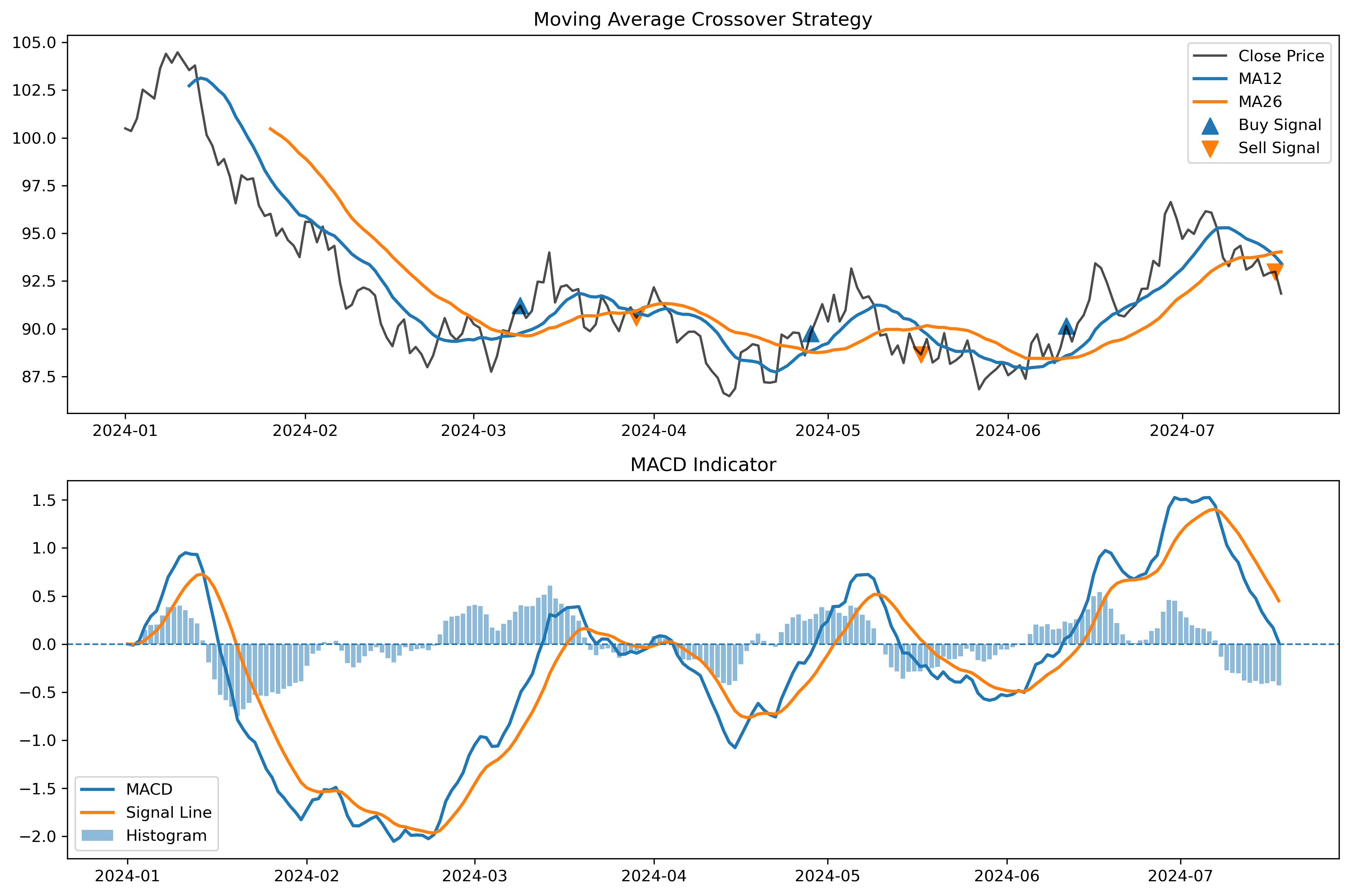

However, crossover systems may also generate false signals during sideways markets.

6.6 Golden Cross and Death Cross¶

Two famous crossover patterns are:

Golden Cross¶

Occurs when:

short moving average crosses above long moving average.

Often interpreted as bullish.

Death Cross¶

Occurs when:

short moving average crosses below long moving average.

Often interpreted as bearish.

This creates a trade-off:

smoother signals,
but delayed reactions.

6.7 MACD: Moving Average Convergence Divergence¶

MACD is one of the most widely used momentum indicators.

It compares:

a short exponential moving average,
and a long exponential moving average.

MACD Formula¶

The MACD line is:

MACD_t = EMA_{short,t} - EMA_{long,t}

Common choices are:

12-day EMA,
26-day EMA.

Signal Line¶

A second moving average is then applied to MACD itself.

This is called the:

signal line

6.8 MACD in Python¶

We now compute and visualize the MACD indicator.

import yfinance as yf
import matplotlib.pyplot as plt

# Download data
sp500 = yf.download(
    "SPY",
    start="2020-01-01",
    auto_adjust=False
)

# Adjusted closing prices
prices = sp500["Adj Close"]

# Exponential moving averages
ema12 = prices.ewm(
    span=12,
    adjust=False
).mean()

ema26 = prices.ewm(
    span=26,
    adjust=False
).mean()

# MACD line
macd = ema12 - ema26

# Signal line
signal = macd.ewm(
    span=9,
    adjust=False
).mean()

# Plot
plt.figure(figsize=(10,5))

plt.plot(
    macd,
    label="MACD",
    linewidth=2
)

plt.plot(
    signal,
    label="Signal Line",
    linewidth=2
)

plt.axhline(
    0,
    linestyle="--",
    linewidth=1
)

plt.title("MACD Indicator")

plt.legend()

plt.show()

6.9 Relative Strength Index (RSI)¶

RSI is a momentum oscillator.

It attempts to measure the speed and magnitude of recent price movements.

RSI usually ranges between:

0 \text{ and } 100

Basic Interpretation¶

RSI	Interpretation
above 70	potentially overbought
below 30	potentially oversold

6.10 RSI Formula¶

RSI is computed from average gains and losses.

The standard formula is:

RSI = 100 - \frac{100}{1+RS}

where:

RS = \frac{\text{Average Gain}}{\text{Average Loss}}

6.11 RSI in Python¶

import yfinance as yf
import pandas as pd
import matplotlib.pyplot as plt

sp500 = yf.download("SPY", start="2020-01-01", auto_adjust=False)

prices = sp500["Adj Close"]

delta = prices.diff()

up = delta.clip(lower=0)
down = -delta.clip(upper=0)

roll_up = up.rolling(14).mean()
roll_down = down.rolling(14).mean()

rs = roll_up / roll_down

rsi = 100 - (100 / (1 + rs))

plt.figure(figsize=(10,4))

plt.plot(rsi)

plt.axhline(70, linestyle="--")
plt.axhline(30, linestyle="--")

plt.title("Relative Strength Index (RSI)")

plt.savefig("figs/ch6/rsi.png", dpi=300, bbox_inches="tight")
plt.close()   # replace with plt.show()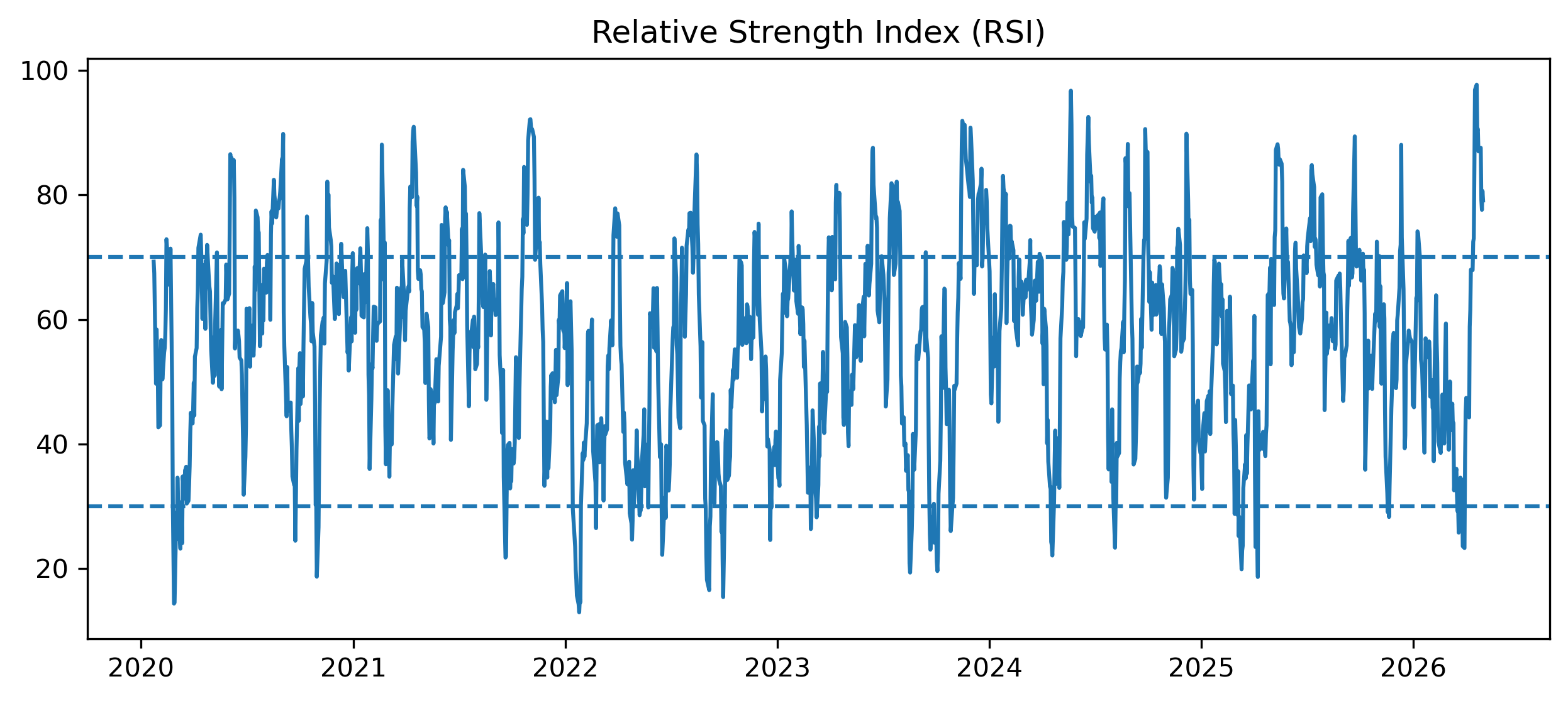

6.12 Bollinger Bands¶

Bollinger Bands combine:

moving averages,
and volatility estimation.

The idea is simple.

If prices move unusually far from their recent average, the movement may be statistically unusual.

Construction¶

Bollinger Bands use:

a moving average,
plus and minus multiples of standard deviation.

Formula¶

Upper band:

MA_t + 2\sigma_t

Lower band:

MA_t - 2\sigma_t

6.13 Bollinger Bands in Python¶

# import yfinance as yf
# import matplotlib.pyplot as plt

# sp500 = yf.download("SPY", start="2020-01-01", auto_adust=False)

# prices = sp500["Adj Close"]

ma20 = prices.rolling(20).mean()
std20 = prices.rolling(20).std()

upper = ma20 + 2 * std20
lower = ma20 - 2 * std20

plt.figure(figsize=(10,5))

plt.plot(prices, label="Price")
plt.plot(ma20, label="20-Day MA")
plt.plot(upper, label="Upper Band")
plt.plot(lower, label="Lower Band")

plt.legend()

plt.title("Bollinger Bands")

plt.savefig("figs/ch6/BB.png", dpi=300, bbox_inches="tight")
plt.close()   # replace with plt.show()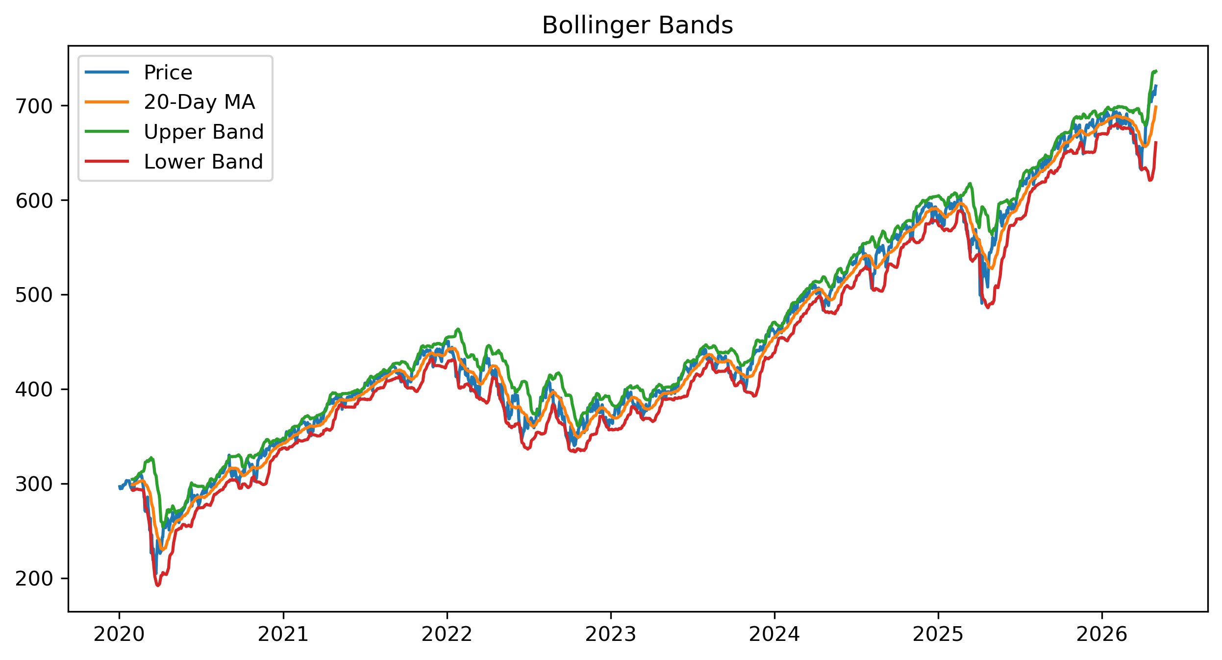

6.14 Indicators as Filters¶

All of these indicators can be interpreted as filters.

Moving Averages¶

Filter short-run noise.

MACD¶

Filters trend changes and momentum.

RSI¶

Filters extreme short-run movements.

Bollinger Bands¶

Filter deviations from recent averages relative to volatility.

6.15 Why Indicators Sometimes Fail¶

Trading indicators are not magic forecasting machines.

They may fail because:

markets are noisy,
trends reverse suddenly,
structural breaks occur,
prices move randomly.

6.16 Trend-Following vs Sideways Markets¶

Many trend-following indicators perform best when strong trends exist.

However, during sideways markets:

false signals may become frequent,
losses may accumulate.

This phenomenon is often called:

whipsaw

6.17 Backtesting¶

Backtesting evaluates how a trading strategy would have performed historically.

Typical steps include:

generating trading signals,
calculating returns,
evaluating cumulative performance.

Historical success may reflect:

luck,
overfitting,
or changing market conditions.

6.18 Simple Backtest Example¶

import yfinance as yf
import pandas as pd
import numpy as np

sp500 = yf.download("SPY", start="2020-01-01", auto_adjust=False)

prices = sp500["Adj Close"]

ma50 = prices.rolling(50).mean()
ma200 = prices.rolling(200).mean()

signal = np.where(ma50 > ma200, 1, 0)

returns = prices.pct_change()

strategy_returns = signal[:-1] * returns[1:]

cumulative = (1 + strategy_returns).cumprod()

cumulative.plot(figsize=(10,4), title="Simple MA Strategy")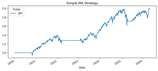

6.19 Long and Short Positions¶

Some trading systems allow:

long positions,
short positions,
or neutral positions.

Long Position¶

Profits when prices rise.

Short Position¶

Profits when prices fall.

6.20 Adjusted Prices in Trading Systems¶

Trading systems should usually use:

Adjusted Close

rather than raw closing prices.

6.21 Overfitting in Trading Strategies¶

A strategy may fit historical data extremely well while performing poorly in the future.

This is called:

overfitting

6.22 Transaction Costs¶

Real trading involves costs such as:

commissions,
bid-ask spreads,
slippage,
taxes.

These costs may substantially reduce profitability.

6.23 Gretl Example: Moving Average Indicator¶

Gretl can construct moving averages easily.

Step 1 — Open Financial Data¶

Load a price series.

Step 2 — Generate Moving Average¶

Menu:

Add → Moving average

Choose the desired window length.

[GRETL Screenshot Placeholder: Moving average indicator]

6.24 Gretl Example: Bollinger Bands¶

Menu:

Variable → Time series plot

Then add:

moving average,
upper and lower volatility bands.

[GRETL Screenshot Placeholder: Bollinger Bands]

6.25 Common Mistakes¶

6.26 Looking Ahead¶

This chapter introduced technical indicators as statistical filters.

The next part of the book begins developing the core theoretical foundations of time series analysis.

We now move toward:

randomness,
dependence,
stationarity,
autocorrelation,
and dynamic models.

Key Takeaways¶

Concept Check¶

Basic¶

What is a trading indicator?
What is the purpose of using indicators in financial markets?
What is a moving average crossover?

Intuition¶

Why do traders use rules (e.g., buy/sell signals) instead of raw data?
What does it mean for an indicator to “filter” a time series?
Why might indicators give different signals on the same data?

Intermediate¶

What is the difference between:
- trend-following indicators
- momentum indicators
What does the RSI measure?
What do Bollinger Bands capture?

Finance Insight¶

Why might simple rules (like moving averages) sometimes work in financial markets?
Why might these rules stop working over time?

Challenge¶

Suppose many traders use the same indicator.

What might happen to its effectiveness?
Why?

Interpretation & Practice¶

A moving average crossover generates a Buy signal.
- What does this suggest about recent price behavior?
- What assumption is the trader making about the future?

A trader uses a very short moving average.
- What type of signals will they get?
- What problem might arise?

A trader uses a very long moving average.
- What type of signals will they get?
- What opportunities might they miss?

RSI indicates an asset is “overbought.”
- What does this mean?
- Does it guarantee that the price will fall?

Bollinger Bands widen significantly.
- What does this indicate about the market?
- What might a trader infer?

A price repeatedly crosses above and below a moving average.
- What kind of market condition does this suggest?
- Why might trading strategies perform poorly here?

Behavioral Insight¶

A trader observes a strong Buy signal and enters the market.
Shortly after, the price reverses.
- What type of risk is this?
- Why do such “false signals” occur?

A strategy performs well historically but fails in recent data.
- What might explain this?
- What does this suggest about financial markets?

Challenge¶

Suppose a price series is purely random (no real trend).
- What signals would trading indicators produce?
- Why is this dangerous?

A trader combines multiple indicators (MA, RSI, Bollinger Bands).

What is the potential benefit?
What is the risk of doing this?

Numerical Practice¶

Extracting Trading Signals¶

Consider the following data:

t	Price	MA(3)
1	100	–
2	102	–
3	101	101.0
4	105	102.7
5	107	104.3
6	104	105.3
7	103	104.7
8	108	105.0

Moving Average Signal¶

Rule:

Buy when Price > MA
Sell when Price < MA

For periods t = 3 to 8:
- Identify Buy / Sell signals.
At which time does the trend appear strongest?

Crossover Strategy¶

Suppose we also have:

t	MA(3)	MA(5)
5	104.3	103.0
6	105.3	103.8
7	104.7	104.2
8	105.0	104.8

Rule:

Buy when MA(3) crosses above MA(5)
Sell when MA(3) crosses below MA(5)

Identify crossover signals.
Why might crossover signals lag behind price movements?

RSI Interpretation (Conceptual)¶

Suppose:

t	RSI
1	30
2	25
3	28
4	40
5	60
6	75
7	80

Rule:

Buy when RSI < 30
Sell when RSI > 70

Identify Buy / Sell signals.
Why might RSI produce false signals in trending markets?

Challenge¶

Suppose a price rises steadily:
100 → 102 → 104 → 106 → 108
- What signals would MA and RSI produce?
- Why might both methods struggle in this case?

Suppose price fluctuates randomly with no trend.
- What problem might arise when applying trading rules?
- What does this suggest about overtrading?

Appendix 6A — Why Exponential Averages Matter in Trading¶

Exponential moving averages place larger weights on recent observations.

This makes them:

more responsive,
faster reacting,
and popular in trading systems.

However, increased responsiveness also increases sensitivity to noise.

Appendix 6B — Trend Following vs Mean Reversion¶

Many trading strategies rely implicitly on one of two beliefs.

Trend Following¶

Prices continue moving in the same direction.

Mean Reversion¶

Prices eventually return toward historical averages.

Financial markets may alternate between:

trending regimes,
and mean-reverting regimes.

This helps explain why no single indicator works perfectly in all market conditions.