Part V Capstone — Forecasting and Model Evaluation

In Part V, we studied:

AR and ARIMA models,
one-step and multi-step forecasting,
static vs dynamic forecasts,
and forecast evaluation.

This capstone applies these ideas to a real time series.

Exercise 1 — Download and Plot Data¶

import yfinance as yf
import numpy as np
import pandas as pd
import matplotlib.pyplot as plt

data = yf.download(
    "SPY",
    start="2018-01-01",
    auto_adjust=False
)

prices = data["Adj Close"].squeeze()

prices.plot(figsize=(10,4))

plt.title("SPY Adjusted Closing Prices")
plt.ylabel("Price")
plt.xlabel("Date")

plt.savefig("figs/ch16_/spy_prices.png", dpi=300, bbox_inches="tight")
plt.close()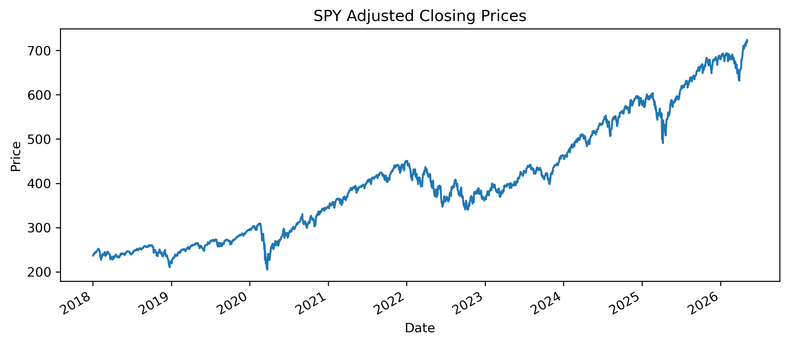

The series shows a clear trend over time.

This suggests that the data may be nonstationary.

Exercise 2 — Compute Returns¶

returns = 100 * np.log(
    prices / prices.shift(1)
)

returns = returns.dropna()

returns.plot(figsize=(10,4))

plt.title("SPY Daily Log Returns")
plt.ylabel("Return (%)")
plt.xlabel("Date")

plt.savefig("figs/ch16_/spy_returns.png", dpi=300, bbox_inches="tight")
plt.close()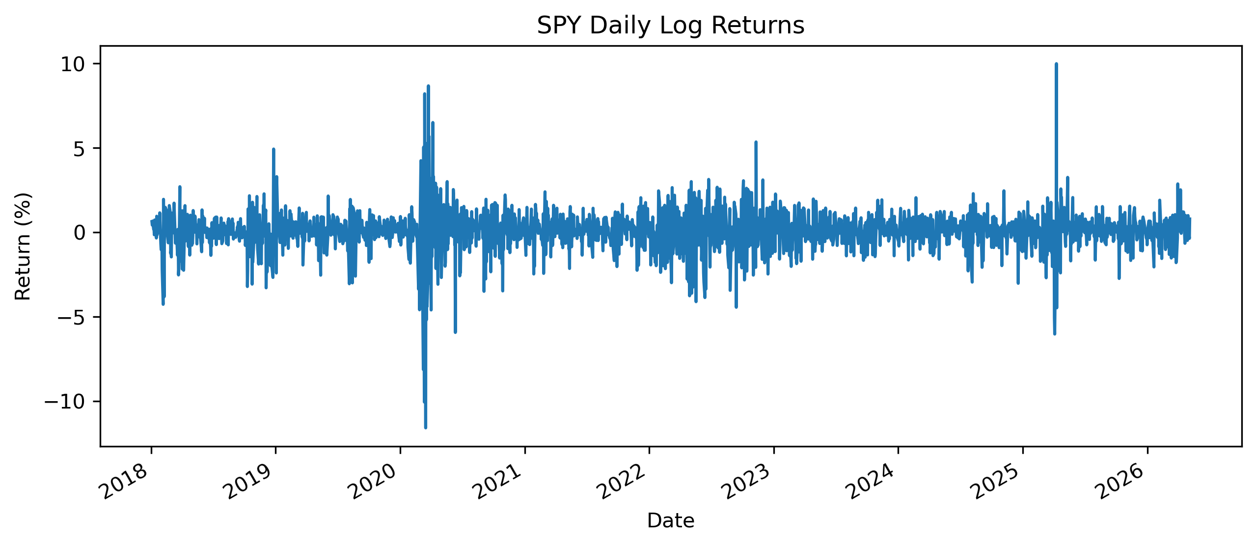

Exercise 3 — Preliminary Analysis¶

Answer the following:

Why are price series often nonstationary while returns are closer to stationary?
What features of the return series are relevant for forecasting?
Would you model prices or returns? Briefly justify your answer.

Exercise 4 — Train, Test, and Holdout Split¶

To evaluate forecasting models properly, we divide the data into three parts:

Training set: used to estimate models
Test set: used to compare models
Holdout set: used for final forecast evaluation

n = len(returns)

train_end = int(0.6 * n)
test_end = int(0.8 * n)

# Split returns
train_r = returns.iloc[:train_end]
test_r = returns.iloc[train_end:test_end]
holdout_r = returns.iloc[test_end:]

# Split prices
train_p = prices.iloc[:train_end+1]
test_p = prices.loc[test_r.index]
holdout_p = prices.loc[holdout_r.index]

# Plot
fig, axes = plt.subplots(2, 1, figsize=(10,6))

# Prices
axes[0].plot(prices)
axes[0].axvline(prices.index[train_end], linestyle=":", linewidth=2)
axes[0].axvline(prices.index[test_end], linestyle=":", linewidth=2)

axes[0].set_title("Price Series (Object of Interest)")
axes[0].set_ylabel("Price")

# Returns
axes[1].plot(returns)
axes[1].axvline(returns.index[train_end], linestyle=":", linewidth=2)
axes[1].axvline(returns.index[test_end], linestyle=":", linewidth=2)

axes[1].set_title("Return Series (Modeling Variable)")
axes[1].set_ylabel("Return (%)")

plt.tight_layout()

plt.savefig("figs/ch16_/split_both_bw.png", dpi=300, bbox_inches="tight")
plt.close()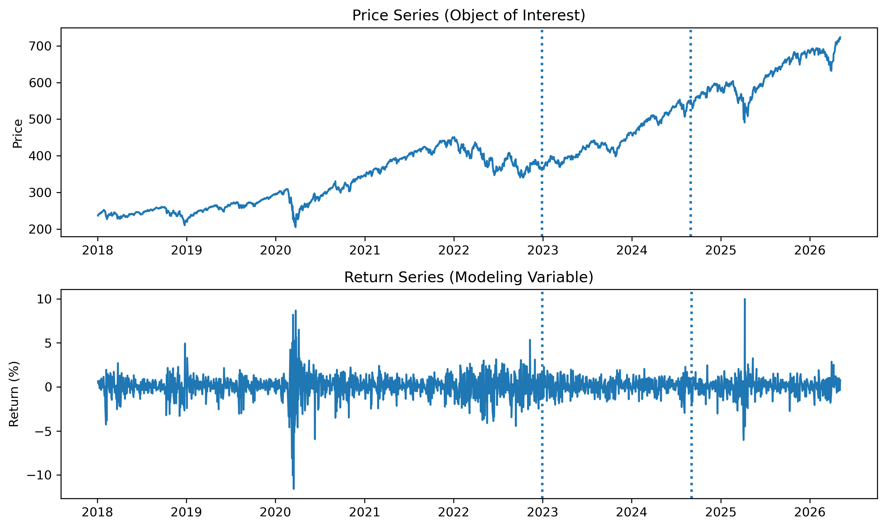

Questions¶

Why are returns typically used for modeling instead of prices?
Why do we still care about forecasting prices?
How are price forecasts related to return forecasts?

Exercise 5 — Stationarity and Diagnostics¶

from statsmodels.tsa.stattools import adfuller

adf_result = adfuller(train_r)

print("ADF Statistic:", adf_result[0])
print("p-value:", adf_result[1])

ADF Statistic: -10.848496749888506
p-value: 1.5502865262934193e-19

from statsmodels.graphics.tsaplots import plot_acf, plot_pacf

fig, axes = plt.subplots(1, 2, figsize=(10,4))

plot_acf(train_r, ax=axes[0], lags=20)
plot_pacf(train_r, ax=axes[1], lags=20)

plt.tight_layout()
plt.savefig("figs/ch16_/acf_pacf.png", dpi=300, bbox_inches="tight")
plt.close()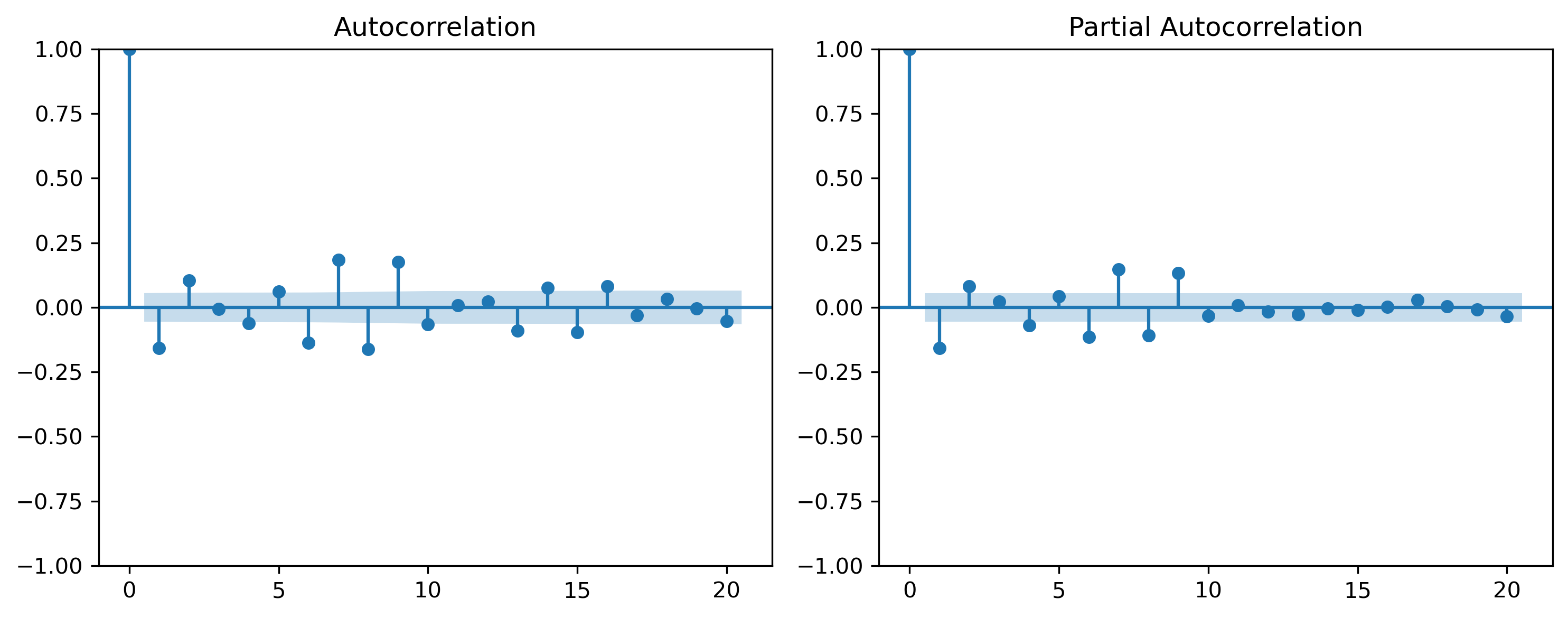

Questions¶

What does the ADF test suggest about stationarity?
Do the ACF/PACF plots clearly suggest a specific model?
Why might model identification be difficult in real data?

Exercise 6 — Two Forecasting Tracks¶

We now compare two forecasting approaches.

Track A — Modeling Returns¶

Returns are usually closer to stationary, so we estimate ARMA-type models on returns.

from statsmodels.tsa.arima.model import ARIMA

# AR(1) on returns
model_ar1_r = ARIMA(train_r, order=(1,0,0))
res_ar1_r = model_ar1_r.fit()

# ARMA(1,1) on returns
model_arma11_r = ARIMA(train_r, order=(1,0,1))
res_arma11_r = model_arma11_r.fit()

print("Return Models")
print("AR(1): AIC =", res_ar1_r.aic, " BIC =", res_ar1_r.bic)
print("ARMA(1,1): AIC =", res_arma11_r.aic, " BIC =", res_arma11_r.bic)

Return Models
AR(1): AIC = 4320.431123957345  BIC = 4335.840573583116
ARMA(1,1): AIC = 4317.4616849387085  BIC = 4338.00761777307

Track B — Modeling Prices¶

Prices are often nonstationary, so we estimate ARIMA models on price levels.

# ARIMA(0,1,0): random walk model for prices
model_rw_p = ARIMA(train_p, order=(0,1,0))
res_rw_p = model_rw_p.fit()

# ARIMA(1,1,1): richer price model
model_arima111_p = ARIMA(train_p, order=(1,1,1))
res_arima111_p = model_arima111_p.fit()

print("Price Models")
print("ARIMA(0,1,0): AIC =", res_rw_p.aic, " BIC =", res_rw_p.bic)
print("ARIMA(1,1,1): AIC =", res_arima111_p.aic, " BIC =", res_arima111_p.bic)

Price Models
ARIMA(0,1,0): AIC = 7134.967174641055  BIC = 7140.103657849645
ARIMA(1,1,1): AIC = 7124.790582801015  BIC = 7140.200032426786

Questions¶

Which return model is preferred by AIC/BIC?
Which price model is preferred by AIC/BIC?
Why should we not compare the AIC/BIC of return models with price models?
What common outcome should we use to compare the two tracks?

Exercise 7 — Forecasting from Both Tracks¶

We now generate forecasts from the best model in each track.

For illustration, suppose:

Track A uses the AR(1) return model.
Track B uses the ARIMA(1,1,1) price model.

Track A — Return Forecasts¶

h = len(test_r)

return_forecast = res_ar1_r.predict(
    start=len(train_r),
    end=len(train_r) + h - 1,
    dynamic=True
)

return_forecast.index = test_r.index

Convert Return Forecasts to Price Forecasts¶

last_train_price = train_p.iloc[-1]

price_forecast_from_returns = []

current_price = last_train_price

for r_hat in return_forecast:
    current_price = current_price * np.exp(r_hat / 100)
    price_forecast_from_returns.append(current_price)

price_forecast_from_returns = pd.Series(
    price_forecast_from_returns,
    index=test_r.index
)

Track B — Direct Price Forecasts¶

price_forecast_arima = res_arima111_p.forecast(
    steps=len(test_r)
)

price_forecast_arima.index = test_r.index

Align Actual Prices¶

actual_test_prices = prices.loc[test_r.index]

Plot Forecasts¶

plt.figure(figsize=(10,5))

plt.plot(actual_test_prices, label="Actual Price", linewidth=2)
plt.plot(price_forecast_from_returns, label="Price Forecast from Return Model", linestyle="--")
plt.plot(price_forecast_arima, label="Direct ARIMA Price Forecast", linestyle=":")

plt.title("Price Forecasts from Two Modeling Tracks")
plt.xlabel("Date")
plt.ylabel("Price")
plt.legend()

plt.savefig("figs/ch16_/two_track_price_forecasts.png", dpi=300, bbox_inches="tight")
plt.close()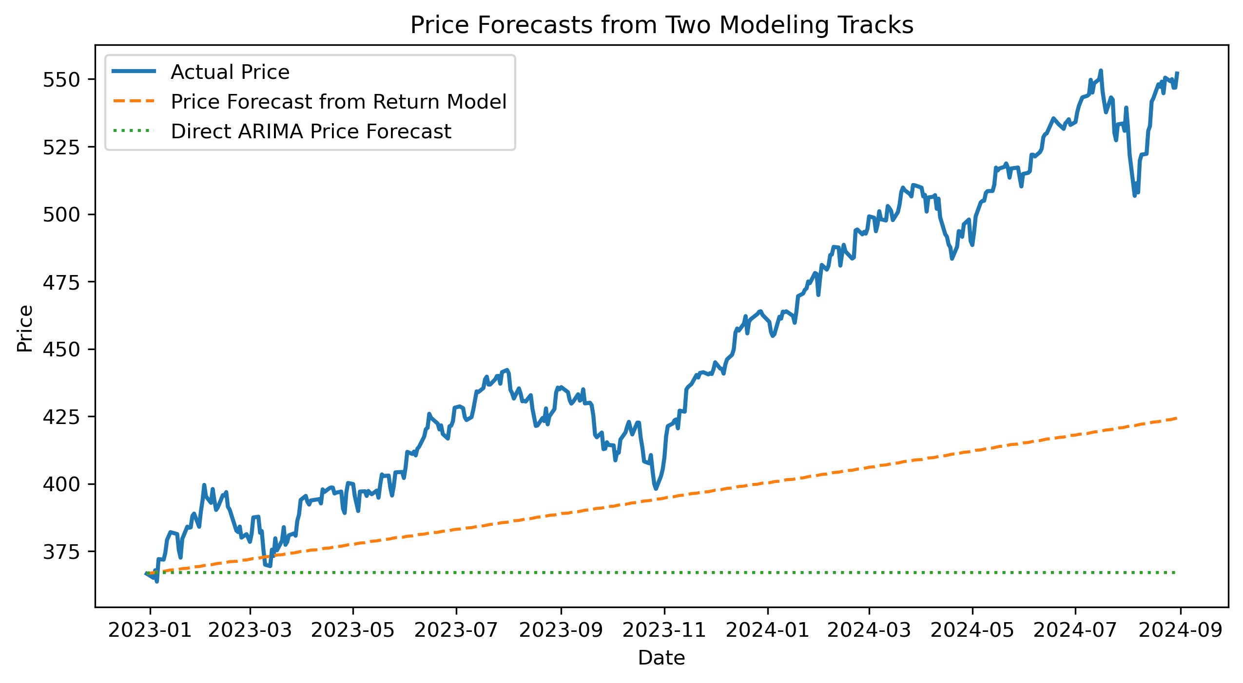

Questions¶

Which forecast tracks actual prices more closely?
Why is this comparison fairer than comparing AIC/BIC across tracks?
What are the advantages of modeling returns first?
What are the advantages of modeling prices directly?

Exercise 8 — Forecast Evaluation Across Tracks¶

We now compare forecast accuracy using the same target variable: price.

def mae(actual, forecast):
    return np.mean(np.abs(actual - forecast))

def rmse(actual, forecast):
    return np.sqrt(np.mean((actual - forecast) ** 2))

mae_return_track = mae(
    actual_test_prices,
    price_forecast_from_returns
)

rmse_return_track = rmse(
    actual_test_prices,
    price_forecast_from_returns
)

mae_price_track = mae(
    actual_test_prices,
    price_forecast_arima
)

rmse_price_track = rmse(
    actual_test_prices,
    price_forecast_arima
)

comparison_table = pd.DataFrame({
    "MAE": [mae_return_track, mae_price_track],
    "RMSE": [rmse_return_track, rmse_price_track]
}, index=[
    "Return Model converted to Price",
    "Direct ARIMA Price Model"
])

comparison_table

| Model                          | MAE       | RMSE      |
|--------------------------------|-----------|-----------|
| Return Model converted to Price| 56.003550 | 67.301639 |
| Direct ARIMA Price Model       | 83.812394 | 99.247644 |

Questions¶

Which track performs better according to MAE?
Which track performs better according to RMSE?
Do both criteria give the same conclusion?
Why might the return-model track and price-model track perform differently?
Which approach would you choose for forecasting prices? Explain.

Exercise 9 — Return-Based Price Forecast with Confidence Band¶

We now forecast returns using the AR(1) return model and convert those forecasts into a price path.

The confidence band is approximate because it is constructed from cumulative return forecast uncertainty.

h = len(test_r)

return_forecast_result = res_ar1_r.get_forecast(
    steps=h
)

return_mean = return_forecast_result.predicted_mean
return_se = return_forecast_result.se_mean

return_mean.index = test_r.index
return_se.index = test_r.index

# Convert returns from percent to decimal
return_mean_dec = return_mean / 100
return_se_dec = return_se / 100

# Cumulative expected log return
cum_return_mean = return_mean_dec.cumsum()

# Approximate cumulative forecast variance
cum_return_var = (return_se_dec ** 2).cumsum()
cum_return_se = np.sqrt(cum_return_var)

# Starting price
last_train_price = train_p.iloc[-1]

# Price forecast path
price_forecast_from_returns = last_train_price * np.exp(cum_return_mean)

# Approximate 95% confidence band
price_lower_from_returns = last_train_price * np.exp(
    cum_return_mean - 1.96 * cum_return_se
)

price_upper_from_returns = last_train_price * np.exp(
    cum_return_mean + 1.96 * cum_return_se
)

actual_test_prices = prices.loc[test_r.index]

plt.figure(figsize=(10,5))

plt.plot(
    actual_test_prices,
    label="Actual Price",
    linewidth=2
)

plt.plot(
    price_forecast_from_returns,
    label="Price Forecast from Return Model",
    linestyle="--"
)

plt.fill_between(
    test_r.index,
    price_lower_from_returns,
    price_upper_from_returns,
    alpha=0.2,
    label="Approximate 95% Forecast Band"
)

plt.title("Return-Based Price Forecast with Confidence Band")
plt.xlabel("Date")
plt.ylabel("Price")
plt.legend()

plt.savefig("figs/ch16_/return_price_forecast_ci.png", dpi=300, bbox_inches="tight")
plt.close()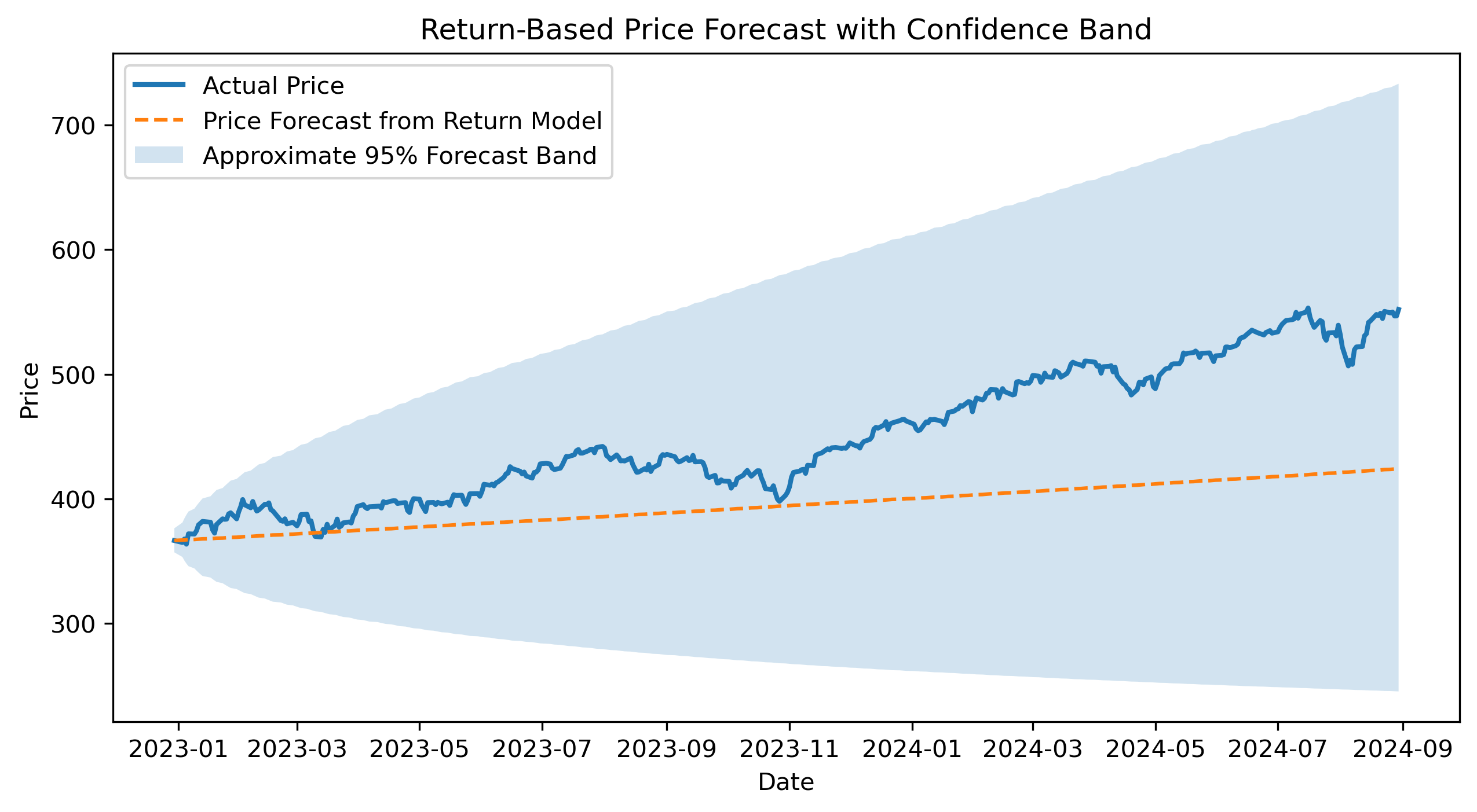

Questions¶

Does the return-based price forecast track the actual price path?
Does the forecast band widen over time?
Why is this confidence band approximate?
Why might small return forecast errors accumulate into larger price forecast errors?

Exercise 10 — Direct ARIMA Price Forecast with Confidence Band¶

We now forecast prices directly using the ARIMA(1,1,1) model.

h = len(test_r)

price_forecast_result = res_arima111_p.get_forecast(
    steps=h
)

price_forecast_arima = price_forecast_result.predicted_mean
price_ci = price_forecast_result.conf_int()

price_forecast_arima.index = test_r.index
price_ci.index = test_r.index

price_lower_arima = price_ci.iloc[:, 0]
price_upper_arima = price_ci.iloc[:, 1]

plt.figure(figsize=(10,5))

plt.plot(
    actual_test_prices,
    label="Actual Price",
    linewidth=2
)

plt.plot(
    price_forecast_arima,
    label="Direct ARIMA Price Forecast",
    linestyle="--"
)

plt.fill_between(
    test_r.index,
    price_lower_arima,
    price_upper_arima,
    alpha=0.2,
    label="Forecast Confidence Band"
)

plt.title("Direct ARIMA Price Forecast with Confidence Band")
plt.xlabel("Date")
plt.ylabel("Price")
plt.legend()

plt.savefig("figs/ch16_/arima_price_forecast_ci.png", dpi=300, bbox_inches="tight")
plt.close()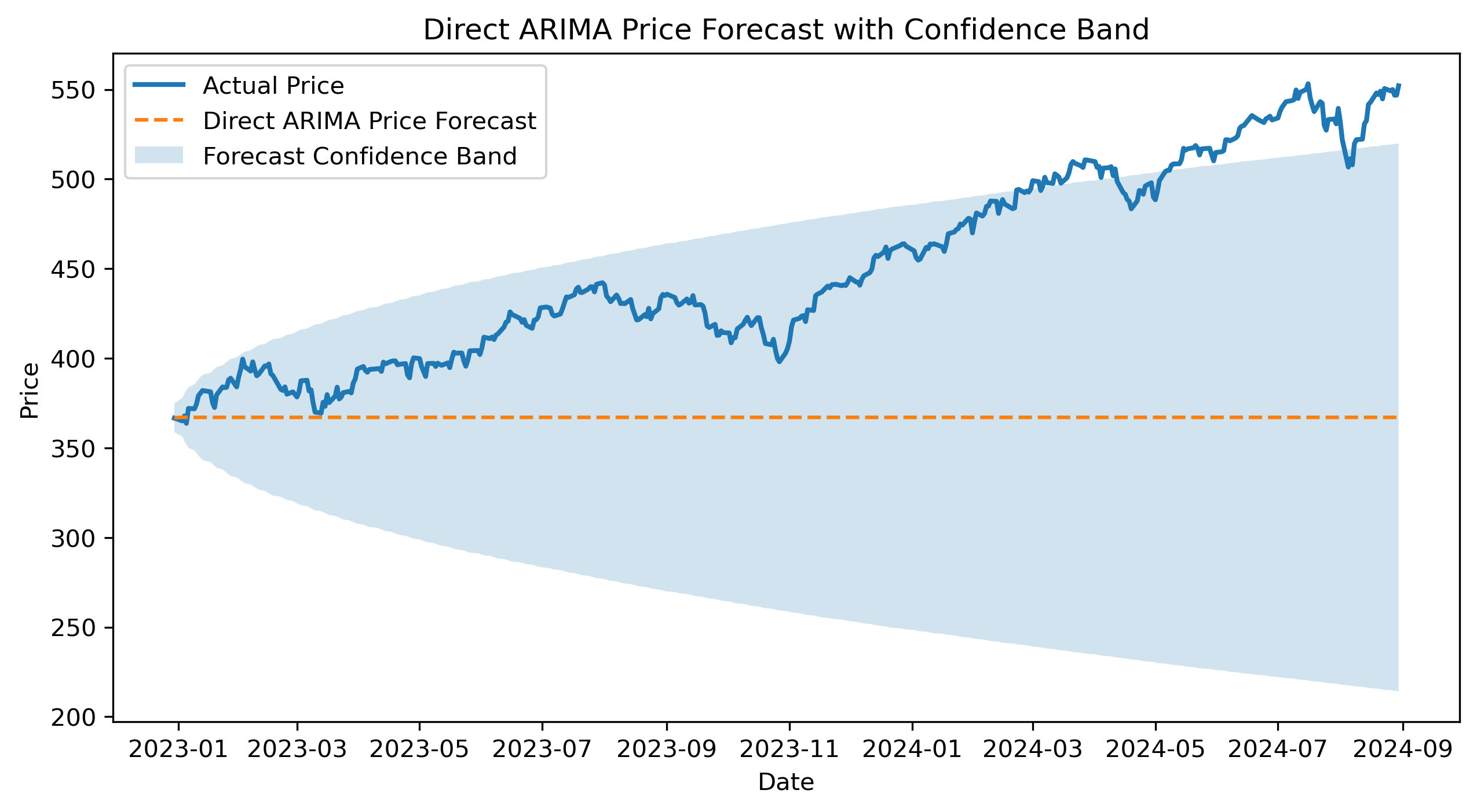

Questions¶

Does the direct ARIMA forecast track the actual price path?
Does the confidence band widen over time?
How does this forecast compare with the return-based price forecast?

Exercise 11 — Comparing Forecast Performance¶

We now compare both forecasting tracks using the same target variable: prices.

summary_table = pd.DataFrame({
    "MAE": [
        mae(actual_test_prices, price_forecast_from_returns),
        mae(actual_test_prices, price_forecast_arima)
    ],
    "RMSE": [
        rmse(actual_test_prices, price_forecast_from_returns),
        rmse(actual_test_prices, price_forecast_arima)
    ],
    "Final Forecast": [
        price_forecast_from_returns.iloc[-1],
        price_forecast_arima.iloc[-1]
    ],
    "Final Actual": [
        actual_test_prices.iloc[-1],
        actual_test_prices.iloc[-1]
    ]
}, index=[
    "Return Model converted to Price",
    "Direct ARIMA Price Model"
])

summary_table

| Model                          | MAE       | RMSE      | Final Forecast | Final Actual |
|--------------------------------|-----------|-----------|----------------|--------------|
| Return Model converted to Price| 56.003550 | 67.301639 | 424.314372     | 552.062988   |
| Direct ARIMA Price Model       | 83.812394 | 99.247644 | 367.039188     | 552.062988   |

Questions¶

Which forecasting approach has the lower MAE?
Which forecasting approach has the lower RMSE?
Do the two evaluation criteria agree?
Which approach would you choose? Explain.
What limitations remain in this comparison?

Challenge (Optional)¶

Compare with a naive forecast.
Compute Theil’s U.
Discuss overfitting vs out-of-sample performance.