Chapter 26 — GARCH Models - Applied Time Series

In the previous chapter, we introduced ARCH models for time-varying volatility.

ARCH models captured an important empirical feature of financial returns:

Large shocks are often followed by large shocks.

Small shocks are often followed by small shocks.

However, ARCH models sometimes require many lag terms to capture realistic volatility persistence.

GARCH models solve this problem by allowing volatility to depend not only on past shocks, but also on past volatility itself.

GARCH models became one of the most influential tools in financial econometrics.

They are widely used in:

risk management,
derivatives pricing,
portfolio analysis,
volatility forecasting,
and algorithmic trading.

Learning Objectives¶

By the end of this chapter, you should be able to:

explain the motivation for GARCH models
distinguish ARCH from GARCH
understand volatility persistence
estimate GARCH models
interpret GARCH coefficients
forecast volatility using GARCH
understand long-run variance
recognize common features of financial volatility

26.1 Why Move Beyond ARCH?¶

Recall the ARCH(1) model:

h_t = \alpha_0 + \alpha_1 e_{t-1}^2

This model explains volatility using past squared shocks.

But real financial volatility often displays very persistent behavior.

A single lag may not be enough.

One solution is to add many ARCH lags:

h_t = \alpha_0 + \alpha_1 e_{t-1}^2 + \alpha_2 e_{t-2}^2 + \cdots + \alpha_q e_{t-q}^2

However, this can become cumbersome.

26.2 The GARCH(1,1) Model¶

The most widely used specification is the GARCH(1,1) model.

Mean Equation¶

Suppose returns follow:

r_t = \mu + e_t

where:

$\mu$ is the mean return,
$e_t$ is the shock.

Variance Equation¶

The GARCH(1,1) variance equation is:

h_t = \omega + \alpha e_{t-1}^2 + \beta h_{t-1}

where:

$h_t$ = conditional variance,
$e_{t-1}^2$ = previous squared shock,
$h_{t-1}$ = previous conditional variance,
$\omega > 0$ ,
$\alpha \ge 0$ ,
$\beta \ge 0$ .

26.3 Interpreting the GARCH Equation¶

The GARCH model combines two forces:

ARCH Component¶

\alpha e_{t-1}^2

captures the impact of recent shocks.

Large shocks increase volatility.

GARCH Component¶

\beta h_{t-1}

captures volatility persistence.

High volatility yesterday tends to imply high volatility today.

This is the defining idea behind GARCH models.

26.4 Volatility Persistence¶

One of the most important features of GARCH models is persistence.

Suppose markets experience a major financial shock.

Volatility often remains elevated for:

days,
weeks,
or even months.

GARCH models capture this gradual decay naturally.

26.5 The Persistence Parameter¶

A key quantity is:

\alpha + \beta

Interpretation¶

Value	Interpretation
small	volatility fades quickly
close to 1	volatility is highly persistent

In financial markets:

\alpha + \beta

is often very close to 1.

26.6 Long-Run Variance¶

For a stable GARCH(1,1) process, the unconditional variance is:

Var(e_t) = \frac{\omega}{1-\alpha-\beta}

provided:

\alpha+\beta < 1

26.7 Volatility Mean Reversion¶

GARCH models imply that volatility tends to revert toward a long-run level.

After periods of turbulence:

volatility gradually declines.

After unusually calm periods:

volatility gradually rises toward normal levels.

26.8 Simulating a GARCH Process¶

We now simulate a GARCH(1,1) process.

import numpy as np
import matplotlib.pyplot as plt

np.random.seed(123)

T = 1000

omega = 0.1
alpha = 0.1
beta = 0.85

e = np.zeros(T)
h = np.zeros(T)

z = np.random.normal(size=T)

h[0] = omega / (1 - alpha - beta)

for t in range(1, T):

    h[t] = (
        omega
        + alpha * e[t-1]**2
        + beta * h[t-1]
    )

    e[t] = np.sqrt(h[t]) * z[t]

plt.figure(figsize=(10,4))

plt.plot(e)

plt.title("Simulated GARCH(1,1) Process")

plt.savefig("figs/ch26/garch.png", dpi=300, bbox_inches="tight")
plt.close()   # replace with plt.show()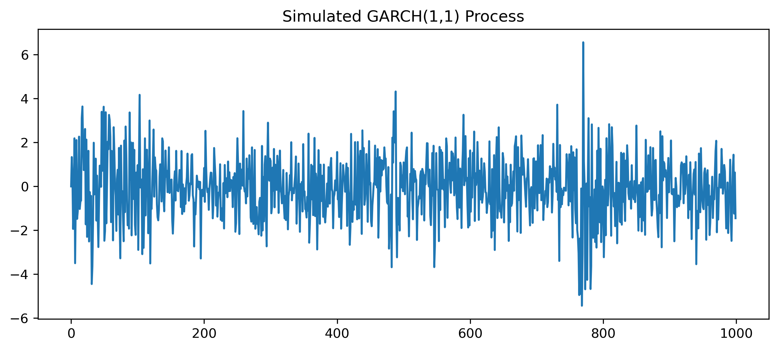

Volatility evolves gradually through time.

26.9 Comparing ARCH and GARCH¶

Feature	ARCH	GARCH
uses past shocks	✓	✓
uses past variance		✓
captures persistence efficiently		✓
requires many lags	often	less often

26.10 Estimating GARCH Models in Python¶

We now estimate a GARCH(1,1) model using real financial data.

import yfinance as yf
import numpy as np
from arch import arch_model

sp500 = yf.download("^GSPC", start="2018-01-01", auto_adjust=False)

returns = 100 * np.log(
    sp500["Adj Close"] /
    sp500["Adj Close"].shift(1)
).dropna()

model = arch_model(
    returns,
    vol="GARCH",
    p=1,
    q=1
)

results = model.fit()

print(results.summary())

[*********************100%***********************]  1 of 1 completed
Iteration:      1,   Func. Count:      6,   Neg. LLF: 13412183422872.883
Iteration:      2,   Func. Count:     15,   Neg. LLF: 1223492784.2470884
Iteration:      3,   Func. Count:     22,   Neg. LLF: 3665.895590631555
Iteration:      4,   Func. Count:     28,   Neg. LLF: 3592.664022773915
Iteration:      5,   Func. Count:     35,   Neg. LLF: 5965.318529783304
Iteration:      6,   Func. Count:     41,   Neg. LLF: 2895.7012213636317
Iteration:      7,   Func. Count:     46,   Neg. LLF: 2895.386785162664
Iteration:      8,   Func. Count:     51,   Neg. LLF: 2895.352625111166
Iteration:      9,   Func. Count:     56,   Neg. LLF: 2895.3516636015643
Iteration:     10,   Func. Count:     61,   Neg. LLF: 2895.351647138695
Iteration:     11,   Func. Count:     66,   Neg. LLF: 2895.351644993276
Iteration:     12,   Func. Count:     70,   Neg. LLF: 2895.3516449937133
Optimization terminated successfully    (Exit mode 0)
            Current function value: 2895.351644993276
            Iterations: 12
            Function evaluations: 70
            Gradient evaluations: 12
                     Constant Mean - GARCH Model Results                      
==============================================================================
Dep. Variable:                  ^GSPC   R-squared:                       0.000
Mean Model:             Constant Mean   Adj. R-squared:                  0.000
Vol Model:                      GARCH   Log-Likelihood:               -2895.35
Distribution:                  Normal   AIC:                           5798.70
Method:            Maximum Likelihood   BIC:                           5821.28
                                        No. Observations:                 2091
Date:                Thu, Apr 30 2026   Df Residuals:                     2090
Time:                        09:59:00   Df Model:                            1
                                Mean Model                                
==========================================================================
                 coef    std err          t      P>|t|    95.0% Conf. Int.
--------------------------------------------------------------------------
mu             0.0874  1.821e-02      4.799  1.592e-06 [5.170e-02,  0.123]
                              Volatility Model                              
============================================================================
                 coef    std err          t      P>|t|      95.0% Conf. Int.
----------------------------------------------------------------------------
omega          0.0508  1.397e-02      3.634  2.785e-04 [2.340e-02,7.817e-02]
alpha[1]       0.1673  2.714e-02      6.164  7.079e-10     [  0.114,  0.221]
beta[1]        0.7960  2.882e-02     27.621 6.164e-168     [  0.740,  0.853]
============================================================================

Covariance estimator: robust

26.11 Interpreting GARCH Output¶

Typical output includes estimates for:

Parameter	Interpretation
$\omega$	baseline variance
$\alpha$	shock effect
$\beta$	volatility persistence

Example¶

Suppose estimates are:

Parameter	Estimate
$\omega$	0.051
$\alpha$	0.167
$\beta$	0.796

Then:

\alpha+\beta=0.963

which implies very persistent volatility.

26.12 Plotting Conditional Volatility¶

We now plot the estimated conditional volatility.

vol = results.conditional_volatility

vol.plot(figsize=(10,4))

plt.title("Estimated GARCH Volatility")

plt.savefig("figs/ch26/garch_vol.png", dpi=300, bbox_inches="tight")
plt.close()   # replace with plt.show()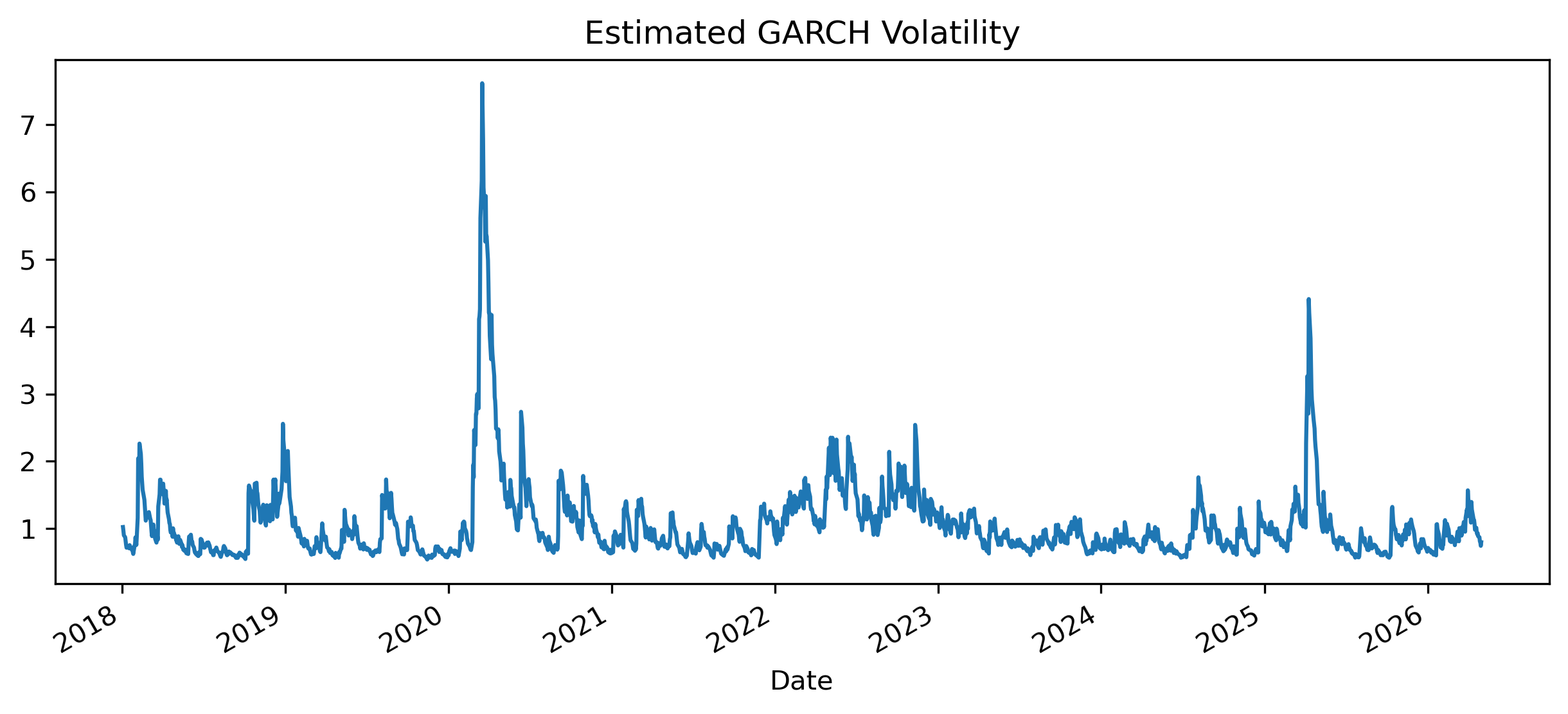

26.13 Volatility Forecasting¶

One of the main applications of GARCH models is volatility forecasting.

Examples include:

Value-at-Risk,
portfolio risk,
derivatives pricing,
stress testing.

26.14 Multi-Step Volatility Forecasts¶

GARCH models can produce forecasts for:

tomorrow’s volatility,
next week’s volatility,
future risk trajectories.

As the forecast horizon increases:

volatility forecasts gradually converge toward long-run variance.

26.15 GARCH and Financial Crises¶

During crises:

shocks become large,
volatility spikes sharply,
persistence increases.

Examples include:

the 2008 Global Financial Crisis,
the COVID-19 market collapse,
cryptocurrency crashes.

Example from Financial Markets¶

[Figure Placeholder: GARCH volatility during financial crisis]

26.16 Fat Tails and GARCH¶

Even if the underlying shocks are normal, GARCH processes often generate:

volatility clustering,
excess kurtosis,
fat tails.

This happens because volatility itself changes through time.

26.17 Limitations of Standard GARCH¶

Standard GARCH models are powerful but imperfect.

They may struggle to capture:

asymmetric volatility,
leverage effects,
sudden structural breaks,
extreme market crashes.

Example: Leverage Effect¶

Negative stock market shocks often increase volatility more than positive shocks.

This motivates extensions such as:

EGARCH,
TGARCH,
GJR-GARCH.

26.18 Gretl Example: Estimating GARCH¶

Gretl provides straightforward tools for GARCH estimation.

Step 1 — Open Data¶

Load a financial return series.

Step 2 — Estimate GARCH¶

Menu:

Model → Time Series → GARCH

Step 3 — Choose Orders¶

For a standard GARCH(1,1):

ARCH order = 1
GARCH order = 1

[GRETL Screenshot Placeholder: GARCH estimation dialog]

Interpreting Gretl Output¶

Typical output includes:

coefficient estimates,
standard errors,
persistence measures,
log-likelihood values.

to ensure variance stability.

26.19 Common Mistakes¶

26.20 Looking Ahead¶

GARCH models provide a powerful framework for modeling financial volatility.

However, financial volatility often displays asymmetry and nonlinear behavior.

More advanced models extend the GARCH framework further.

Key Takeaways¶

Concept Check¶

Basic¶

What is a GARCH model?
How does GARCH differ from ARCH?
What does the variance equation represent?

Intuition¶

What does it mean to say “volatility has memory”?
Why do financial markets exhibit persistent volatility?
Why is it unrealistic to assume constant variance?

Structure¶

In the GARCH(1,1) model:
- what does $\alpha$ represent?
- what does $\beta$ represent?
Why are both components needed?

Persistence¶

What does the quantity $\alpha + \beta$ measure?
What does it mean if $\alpha + \beta$ is close to 1?

Long-Run Behavior¶

What is the long-run variance?
Why does volatility revert toward a long-run level?

Challenge¶

Can volatility be highly persistent even if shocks are short-lived?

Interpretation & Practice¶

A GARCH model estimates:

$\alpha = 0.1$
$\beta = 0.85$
- What does this imply about persistence?

A large shock occurs in the market.

What does the GARCH model predict for future volatility?

Volatility declines slowly after a crisis.

What does this suggest about $\beta$ ?

$\alpha$ is large but $\beta$ is small.

What does this imply?

$\beta$ is large but $\alpha$ is small.

What does this imply?

Mean Reversion¶

Why does volatility eventually return to a long-run level?

Economic Interpretation¶

Why is volatility persistence important for risk management?

Challenge¶

Why might a GARCH model produce fat tails even with normal shocks?
Why might negative returns increase volatility more than positive returns? What real-world behavior does this reflect?

Numerical Practice¶

GARCH Equation¶

Suppose:

h_t = 0.1 + 0.2 e_{t-1}^2 + 0.7 h_{t-1}

and:

$e_{t-1} = 2$
$h_{t-1} = 1$

Compute $h_t$ .

Persistence¶

Compute:

\alpha + \beta

What does this imply?

Long-Run Variance¶

Suppose:

\omega = 0.1, \quad \alpha = 0.2, \quad \beta = 0.7

Compute long-run variance:

\frac{\omega}{1 - \alpha - \beta}

Interpretation¶

If $\alpha + \beta = 0.98$ :

what does this imply?

Stability¶

What happens if:

\alpha + \beta \ge 1

Forecasting¶

Why do volatility forecasts converge to long-run variance?

Challenge¶

Suppose volatility is very persistent.

What does this imply about risk forecasting?

You estimate a GARCH(1,1) model for stock returns and find:

$\alpha = 0.15$
$\beta = 0.80$

Is volatility persistent?
How quickly does it decay?
What does this imply for risk management?

Graph Interpretation¶

Consider a GARCH volatility plot showing:

large spikes during crises
slow decline afterward

What does this suggest about volatility persistence?
Why does volatility not drop immediately?
What does this imply about $\beta$ ?

Comparison¶

Compare two series:

one where volatility drops quickly
one where volatility persists

Which has higher $\alpha + \beta$ ?

Challenge¶

Why is volatility easier to observe than to predict precisely?

Appendix 26A — Stability Condition for GARCH(1,1)¶

For the GARCH(1,1) model:

h_t = \omega + \alpha e_{t-1}^2 + \beta h_{t-1}

the stability condition is:

\alpha+\beta<1

Why This Matters¶

If:

\alpha+\beta \ge 1

then volatility shocks may never decay fully.

Variance may become nonstationary or explosive.

is to 1, the more persistent volatility becomes.

Appendix 26B — ARCH vs GARCH Intuition¶

ARCH models say:

Volatility depends on recent shocks.

GARCH models add:

Volatility also depends on past volatility itself.

This additional persistence greatly improves empirical realism.

Appendix 26C — Extensions of GARCH Models¶

Standard GARCH models assume that positive and negative shocks have the same effect on volatility.

In financial markets, this is often unrealistic.

This phenomenon is known as the leverage effect.

C.1 Why Extensions Are Needed¶

Empirical evidence shows:

stock market declines → sharp increase in volatility
stock market increases → smaller effect

Standard GARCH cannot capture this asymmetry.

C.2 GJR-GARCH Model¶

The GJR-GARCH model introduces asymmetry:

h_t = \omega + \alpha e_{t-1}^2 + \gamma e_{t-1}^2 I(e_{t-1}<0) + \beta h_{t-1}

where:

$I(e_{t-1}<0)$ is an indicator for negative shocks

C.3 EGARCH Model¶

The EGARCH model uses a logarithmic specification:

\log h_t = \omega + \beta \log h_{t-1} + \alpha \frac{e_{t-1}}{\sqrt{h_{t-1}}} + \gamma \left|\frac{e_{t-1}}{\sqrt{h_{t-1}}}\right|

C.4 T-GARCH (Threshold GARCH)¶

T-GARCH models also capture asymmetric responses:

volatility behaves differently depending on shock size or sign

C.5 Key Takeaways¶

C.6 Practical Insight¶

C.7 When to Use Extensions¶

Consider extensions when:

markets show strong crash behavior
negative shocks dominate volatility
risk management is critical

C.8 Looking Ahead¶

Advanced volatility models are widely used in:

option pricing
portfolio risk
stress testing

Understanding asymmetry is essential for realistic financial modeling.