Chapter 7 — Randomness and Dependence

In earlier chapters, we explored financial returns, smoothing methods, and trading indicators. We now begin developing the core ideas of time series analysis more formally.

A central insight of time series analysis is that observations collected over time are often dependent. What happens today may be related to what happened yesterday, last week, or even many periods ago.

This chapter introduces:

stochastic processes
white noise
dependence across time
persistence
random walks

These ideas form the conceptual foundation for later chapters on stationarity, ARIMA models, forecasting, and cointegration.

Learning Objectives¶

By the end of this chapter, you should be able to:

explain what a time series is
distinguish randomness from dependence
understand white noise processes
interpret persistence in economic and financial data
understand the random walk model
simulate and visualize simple stochastic processes

7.1 What Is a Time Series?¶

Examples include:

daily stock prices
quarterly GDP
monthly inflation
exchange rates
unemployment rates
rainfall measurements

A time series can be written as:

X_t = \{x_1, x_2, \dots, x_T\}

(1)

where:

$t$ indexes time
$x_t$ is the observation at time $t$

For example:

inflation this month is related to inflation last month
stock prices today are related to yesterday’s prices
GDP evolves gradually over time

7.2 Stochastic Processes¶

A time series is usually viewed as a realization of a stochastic process.

We observe only one realization of the process:

x_1, x_2, \dots, x_T

(2)

but we imagine that these observations are generated by an underlying probabilistic mechanism.

7.3 Randomness and Dependence¶

In statistics, we often study random variables independently. In time series analysis, however, the timing of observations matters.

Two key questions arise:

How random is the process?
How dependent are observations over time?

Example: Daily Stock Returns¶

Daily returns appear highly random:

difficult to predict exactly
fluctuate around zero
heavily influenced by news and expectations

But even highly random processes may still exhibit:

persistence
volatility clustering
serial dependence

7.4 White Noise¶

The simplest stochastic process is white noise.

Thus:

mean is constant
variance is constant
observations are uncorrelated over time

We often write:

w_t \sim wn(0,\sigma_w^2)

(3)

7.5 Simulating White Noise¶

import numpy as np
import matplotlib.pyplot as plt

np.random.seed(10101)

wn = np.random.normal(0, 2, 500)

plt.figure(figsize=(10,4))
plt.plot(wn, lw=1)
plt.title("Simulated White Noise")
plt.xlabel("Time")
plt.ylabel("$w_t$")

plt.savefig("figs/ch7/wn.png", dpi=300, bbox_inches="tight")
plt.close()   # replace with plt.show()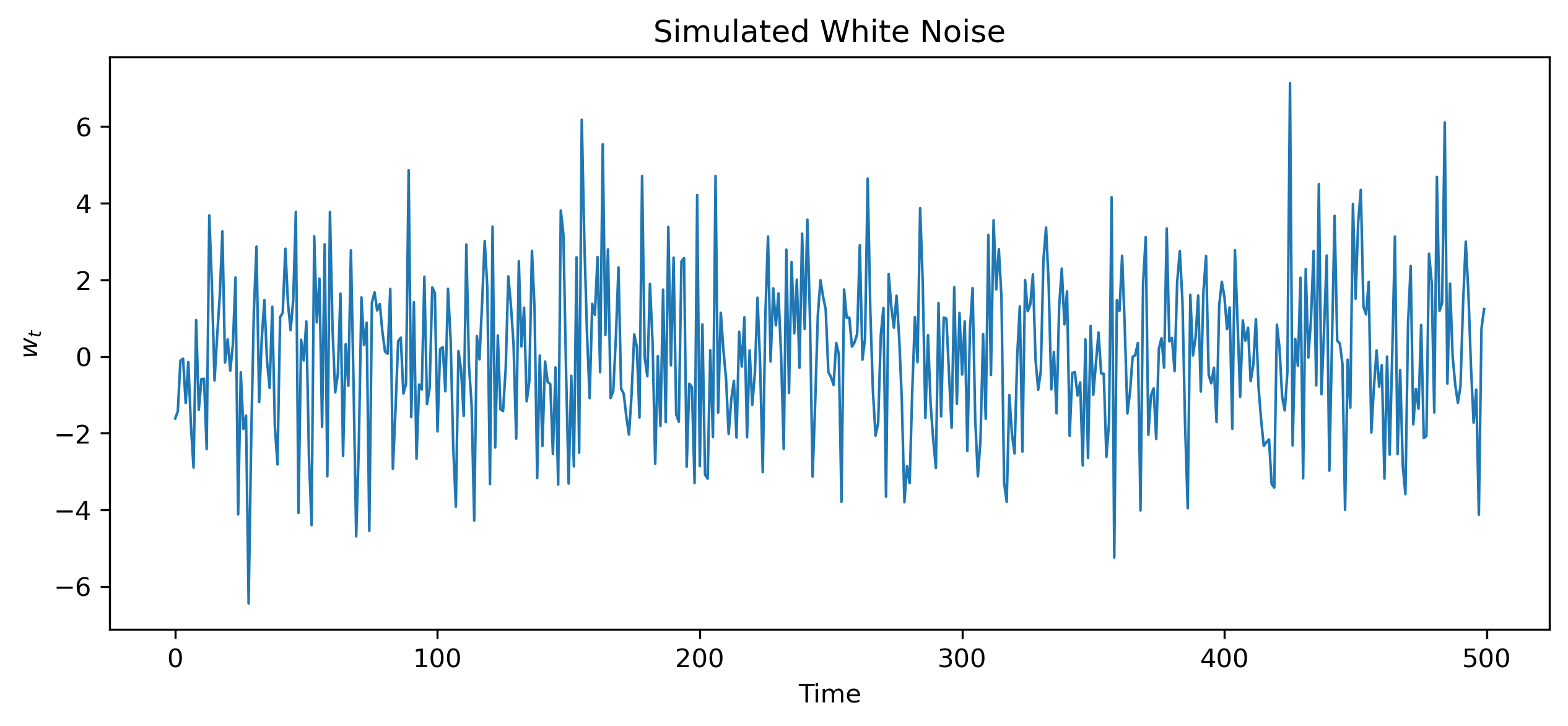

7.6 Gaussian White Noise¶

If white noise is normally distributed, we call it Gaussian white noise.

w_t \sim N(0,\sigma_w^2)

(4)

Gaussian white noise is widely used in theoretical models because it is mathematically convenient.

7.7 Covariance and Correlation¶

To study dependence across time, we first review covariance and correlation.

Variance¶

Var(X) = E[(X - \mu_X)^2]

(5)

Covariance¶

Cov(X,Y) = E[(X-\mu_X)(Y-\mu_Y)]

(6)

Correlation¶

Corr(X,Y) = \frac{Cov(X,Y)} {\sqrt{Var(X)}\sqrt{Var(Y)}}

(7)

7.8 Dependence Across Time¶

In time series analysis, we are interested in relationships such as:

Cov(X_t, X_{t-1})

Cov(X_t, X_{t-2})

and more generally:

Cov(X_t, X_{t-h})

where $h$ is called the lag.

7.9 Persistence¶

Some time series exhibit strong persistence.

Examples:

inflation
interest rates
exchange rates
stock prices

In persistent series:

shocks may have long-lasting effects
observations change gradually over time

7.10 Random Walks¶

One of the most important models in time series analysis is the random walk.

Interpretation¶

Each new observation equals:

the previous value
plus a random shock

7.11 Simulating a Random Walk¶

np.random.seed(123)

w = np.random.normal(0, 1, 500)
x = np.cumsum(w)

plt.figure(figsize=(10,4))
plt.plot(x, lw=1)
plt.title("Simulated Random Walk")
plt.xlabel("Time")
plt.ylabel("$x_t$")

plt.savefig("figs/ch7/rw.png", dpi=300, bbox_inches="tight")
plt.close()   # replace with plt.show()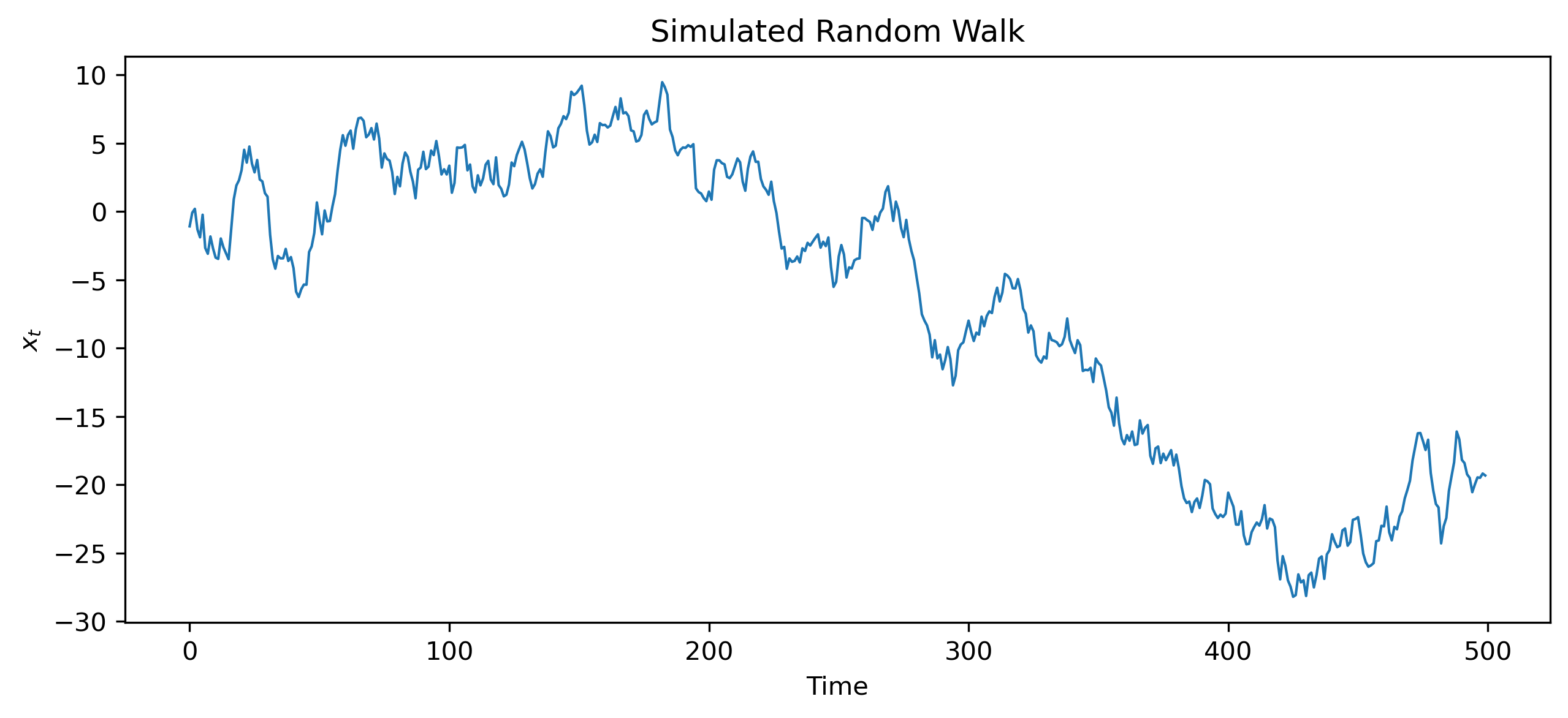

7.12 White Noise vs Random Walk¶

Feature	White Noise	Random Walk
Mean reverting	Yes	No
Persistent	No	Yes
Variance constant	Yes	No
Predictable structure	None	Strong persistence

7.13 Why Random Walks Matter¶

Random walks play a central role in economics and finance.

Examples include:

stock prices
exchange rates
some macroeconomic aggregates

Financial Interpretation¶

If stock prices follow a random walk:

past price movements contain little forecasting power
price changes are difficult to predict systematically

This idea is closely related to the efficient market hypothesis.

7.14 Looking Ahead¶

In this chapter, we introduced:

stochastic processes
white noise
dependence
persistence
random walks

These ideas naturally lead to the concept of stationarity, which we study in the next chapter.

Key Takeaways¶

Concept Check¶

Basic¶

What is a stochastic process?
What is white noise?
What is a random walk?

Intuition¶

Why are observations in a time series typically not independent?
What does it mean for a series to exhibit persistence?
Why is white noise considered unpredictable?

Intermediate¶

What is serial dependence?
What is a lag in time series analysis?
Why can a random walk look like it has a trend even if it does not?

Finance Insight¶

Why might stock prices behave like a random walk?
What does this imply about the ability to predict future prices?

Challenge¶

Suppose a series looks smooth and trending.

Does this imply it is predictable?
Why or why not?

Interpretation & Practice¶

Consider a white noise series.
- What pattern would you expect to see in a plot?
- Why is it difficult to forecast?

Consider a random walk.
- Why does it appear to drift over time?
- What role do past shocks play?

A series shows strong persistence.
- What does this imply about the effect of shocks?
- How might this affect forecasting?

A plot shows large swings but no clear pattern.
- Is this more likely white noise or a random walk?
- Why?

A time series appears to trend upward.
- What are two possible explanations?
- Why must we be careful in interpreting this?

Behavioral Insight¶

A trader believes that an upward trend will continue.
- What assumption are they making about dependence?
- Why might this be misleading?

Challenge¶

Suppose you simulate two series:
- Series A: white noise
- Series B: random walk
- Which one is easier to predict?
- Why?

Numerical Practice¶

White Noise vs Random Walk¶

Suppose you observe the following values:
Series A:
2, −1, 1, −2, 0, 1
Series B:
2, 1, 2, 0, 0, 1
- Which series looks more like white noise?
- Which looks more persistent?

Step-by-Step Random Walk¶

Suppose a random walk is defined as:

[ x_t = x_{t-1} + w_t ]

with:

initial value (x_0 = 100)
shocks (w_t): 2, −1, 3, −2

Compute (x_1, x_2, x_3, x_4)

What do you notice about how shocks affect the series?

Variance Intuition¶

Consider two processes:

white noise
random walk

Which one has constant variance over time?
Which one becomes more volatile as time increases?
Why?

Persistence¶

Suppose a shock of +5 occurs in:

a white noise process
a random walk

How long does the effect last in each case?

Challenge¶

Suppose you observe a series that behaves like a random walk.

Why might differencing the series remove persistence?
What do you expect the differenced series to look like?