Chapter 5 — Smoothing and Trend Estimation

Real-world time series are often noisy.

Daily stock prices fluctuate constantly.

Macroeconomic indicators rise and fall irregularly.

Even when underlying trends exist, short-run variation can obscure them.

One of the central goals of time series analysis is therefore:

This chapter introduces several important smoothing and trend estimation methods.

We study:

moving averages,
exponential smoothing,
Holt and Holt–Winters methods,
LOESS smoothing,
splines,
the HP filter,
and the bias–variance trade-off.

The emphasis throughout is intuition-first and applications-oriented.

All these methods answer the same question: how do we separate signal from noise?

Learning Objectives¶

By the end of this chapter, you should be able to:

explain the purpose of smoothing
distinguish signal from noise
construct moving averages
understand exponential smoothing intuitively
explain Holt and Holt–Winters methods
understand local smoothing methods such as LOESS
interpret HP-filter trends
understand the bias–variance trade-off
apply smoothing methods using Python and GRETL

5.1 Why Smooth Data?¶

Many time series contain substantial short-run noise.

Examples include:

daily stock returns,
exchange rates,
cryptocurrency prices,
high-frequency macroeconomic indicators.

Random fluctuations can make it difficult to see broader patterns.

5.2 Signal and Noise¶

A useful conceptual framework is:

\text{Observed Series} = \text{Signal} + \text{Noise}

where:

signal = meaningful structure,
noise = random fluctuations.

Example¶

Suppose stock prices fluctuate daily because of:

random news,
speculation,
temporary shocks.

Despite this noise, the market may still exhibit:

long-run trends,
business cycles,
persistent movements.

Smoothing attempts to recover these underlying components.

5.3 Moving Averages¶

One of the simplest smoothing methods is the moving average.

A moving average replaces each observation with an average of nearby observations.

Simple Moving Average¶

A $k$ -period moving average is:

MA_t = \frac{1}{k} \sum_{i=0}^{k-1}x_{t-i}

where:

$k$ = window length,
$x_t$ = observed series.

5.4 Example: 5-Day Moving Average¶

Suppose stock prices are:

Day	Price
1	100
2	102
3	101
4	104
5	103

The 5-day moving average is:

\frac{100+102+101+104+103}{5} = 102

5.5 Moving Averages in Python¶

We now compute a moving average using Python.

import yfinance as yf
import matplotlib.pyplot as plt

aapl = yf.download("AAPL", start="2020-01-01", auto_adjust=False)

prices = aapl["Adj Close"]

ma50 = prices.rolling(50).mean()

plt.figure(figsize=(10,4))

plt.plot(prices, label="Price")

plt.plot(ma50, label="50-Day MA")

plt.legend()

plt.title("Apple Stock Price and 50-Day Moving Average")

plt.savefig("figs/ch5/MA.png", dpi=300, bbox_inches="tight")
plt.close()   # replace with plt.show()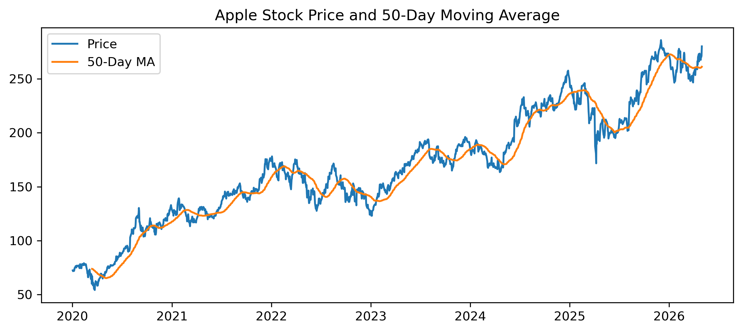

5.6 Choosing the Window Length¶

The smoothing effect depends heavily on the window length.

Small Window¶

responds quickly,
less smooth,
more sensitive to noise.

Large Window¶

smoother,
slower response,
may miss turning points.

5.7 Moving Averages as Filters¶

Moving averages act as filters.

They suppress:

high-frequency fluctuations,
short-run noise.

At the same time, they preserve:

lower-frequency movements,
trends,
cycles.

This becomes especially important in:

spectral analysis,
trading indicators,
signal extraction.

5.8 Exponential Smoothing¶

Moving averages assign equal weight to all observations inside the window.

Exponential smoothing instead assigns:

larger weights to recent observations,
smaller weights to older observations.

Simple Exponential Smoothing¶

The updating equation is:

\hat x_{t+1} = \alpha x_t + (1-\alpha)\hat x_t

where:

$0<\alpha<1$ ,
$\alpha$ controls responsiveness.

Alternative Form (Error-Correction View)¶

The updating equation can also be written as:

\hat x_{t+1} = \hat x_t + \alpha(x_t - \hat x_t)

5.9 Interpreting the Smoothing Parameter¶

The parameter:

\alpha

controls how quickly the model reacts to new information.

Large $\alpha$ ¶

reacts quickly,
more sensitive to recent changes,
less smooth.

Small $\alpha$ ¶

smoother,
reacts slowly,
emphasizes long-run behavior.

5.10 Exponential Smoothing in Python¶

import yfinance as yf
import matplotlib.pyplot as plt

aapl = yf.download("AAPL", start="2020-01-01", auto_adjust=False)

prices = aapl["Adj Close"]

ewma = prices.ewm(span=50).mean()

plt.figure(figsize=(10,4))

plt.plot(prices, label="Price")

plt.plot(ewma, label="EWMA")

plt.legend()

plt.title("Exponential Smoothing")

plt.savefig("figs/ch5/ema.png", dpi=300, bbox_inches="tight")
plt.close()   # replace with plt.show()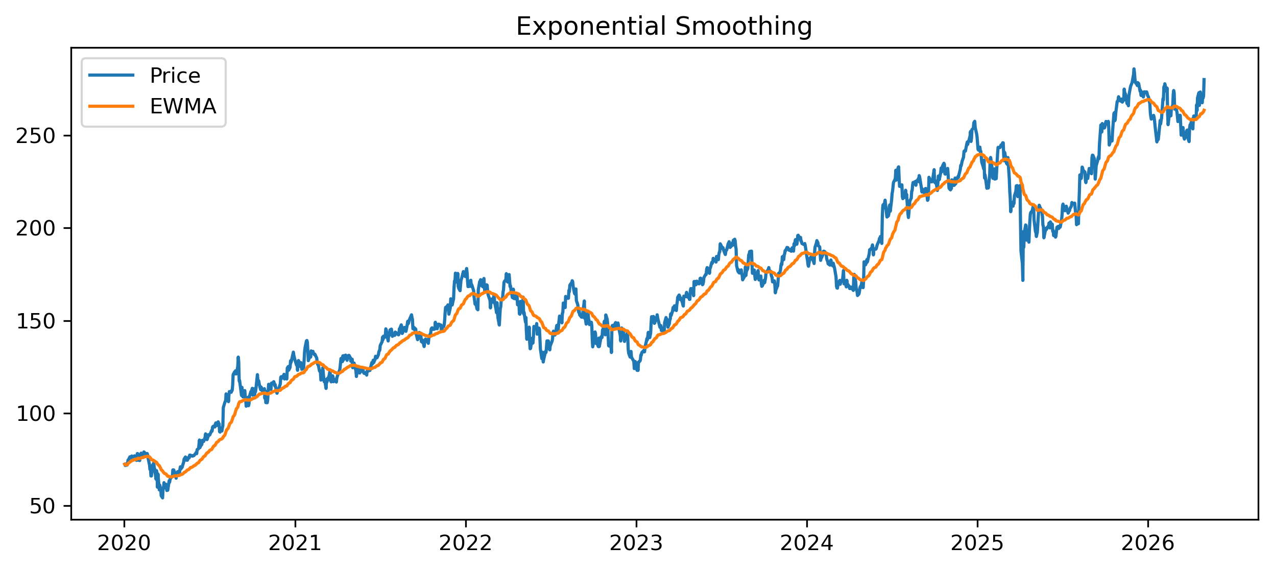

5.11 Forecasting Interpretation¶

Exponential smoothing is not only a smoothing method.

It is also a forecasting method.

The smoothed series itself becomes a forecast of future values.

5.12 Holt’s Method¶

Simple exponential smoothing works best when no trend exists.

But many economic time series trend through time.

Holt’s method extends exponential smoothing by modeling:

level,
and trend.

Holt Updating Equations¶

Level¶

\ell_t = \alpha x_t + (1-\alpha)(\ell_{t-1}+b_{t-1})

Trend¶

b_t = \beta(\ell_t-\ell_{t-1}) + (1-\beta)b_{t-1}

5.13 Holt–Winters Method¶

Some time series contain:

trend,
and seasonality.

Holt–Winters methods extend Holt’s method further to model seasonal structure.

Examples include:

tourism,
electricity demand,
retail sales.

5.14 Example: Seasonal Data¶

import pandas as pd
import matplotlib.pyplot as plt

url = "https://raw.githubusercontent.com/jbrownlee/Datasets/master/airline-passengers.csv"

df = pd.read_csv(url)

df["Passengers"].plot(figsize=(10,4))

plt.title("Monthly Airline Passengers")

plt.savefig("figs/ch5/airline.png", dpi=300, bbox_inches="tight")
plt.close()   # replace with plt.show()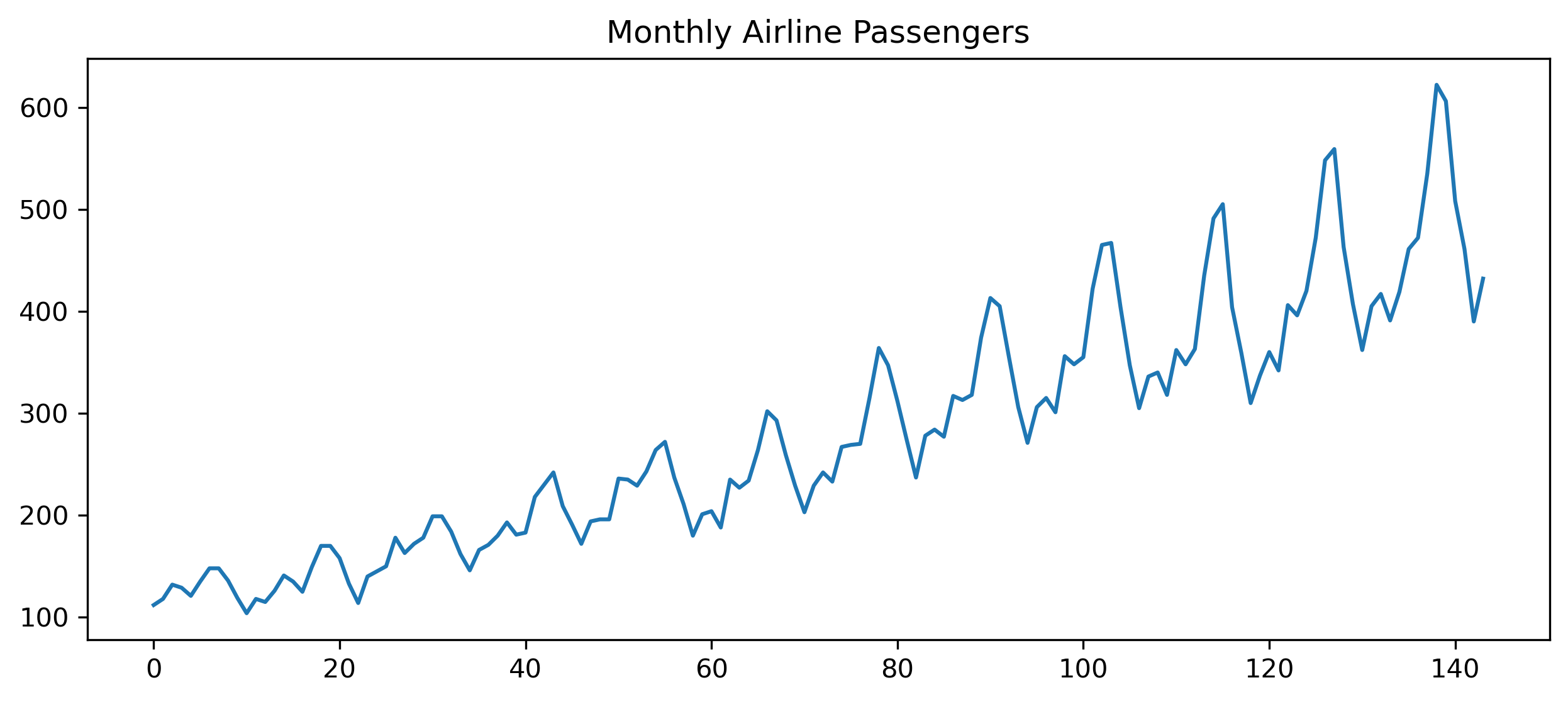

5.15 Local Smoothing: LOESS¶

LOESS (Locally Weighted Scatterplot Smoothing) is a flexible smoothing method.

Instead of fitting one global trend, LOESS fits:

many local regressions.

This makes LOESS useful when trends change gradually over time.

5.16 LOESS Example in Python¶

import numpy as np
import matplotlib.pyplot as plt
from statsmodels.nonparametric.smoothers_lowess import lowess

np.random.seed(123)

x = np.arange(200)

y = (
    0.05*x
    + np.sin(x/10)
    + np.random.normal(scale=1,size=200)
)

smooth = lowess(y, x, frac=0.1)

plt.figure(figsize=(10,4))

plt.plot(x, y, alpha=0.5)

plt.plot(smooth[:,0], smooth[:,1])

plt.title("LOESS Smoothing")

plt.savefig("figs/ch5/loess.png", dpi=300, bbox_inches="tight")
plt.close()   # replace with plt.show()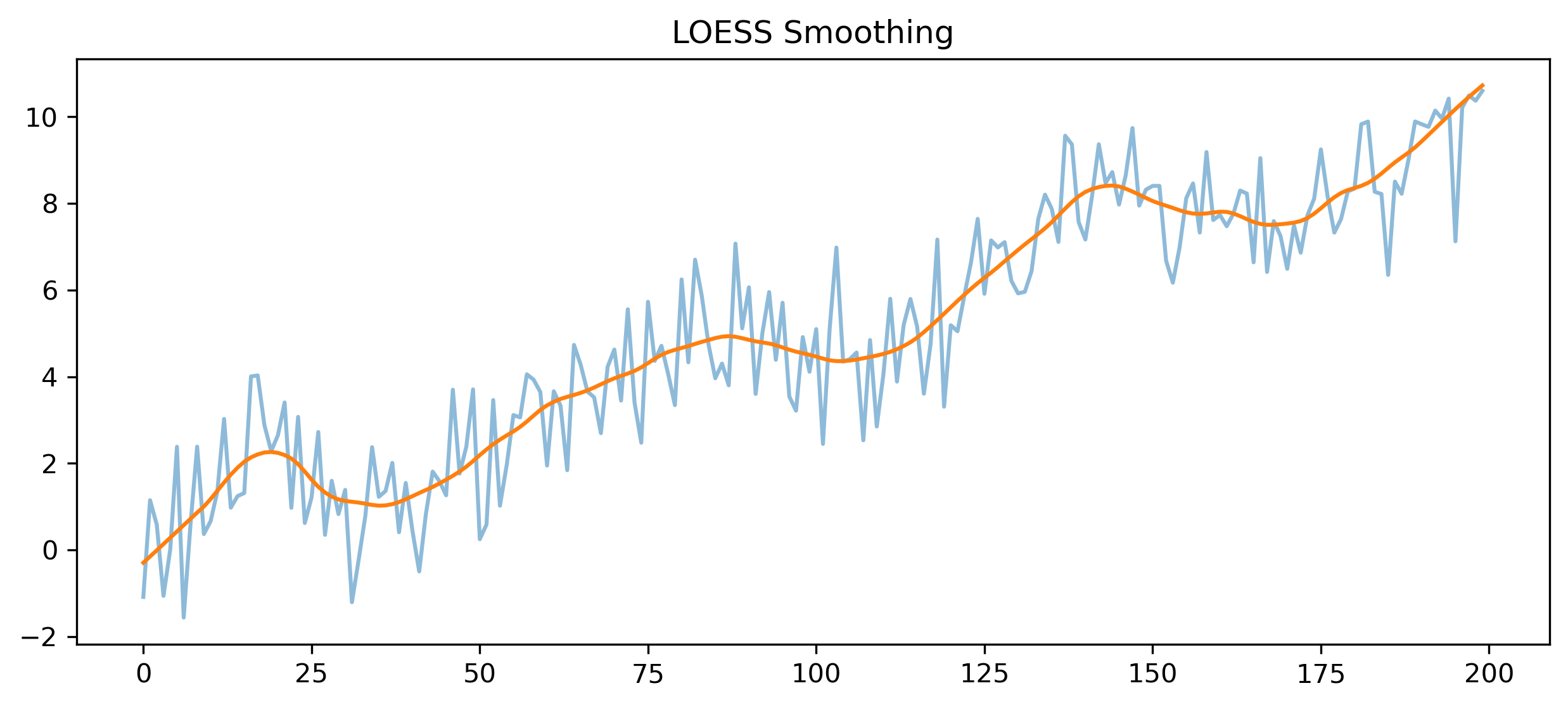

5.17 Splines¶

Splines provide a flexible way to model smooth trends in a time series.

Instead of fitting a single curve to the entire dataset, splines divide the data into segments and fit simple curves to each part.

Intuition¶

A spline works like a flexible ruler:

it bends to follow the data,
but remains smooth,
and avoids sharp, unrealistic jumps.

Why Not Use One Polynomial?¶

Fitting a single high-degree polynomial can lead to:

extreme oscillations,
poor behavior at the edges,
overfitting.

Splines solve this by:

breaking the data into smaller regions,
fitting simpler curves locally,
ensuring smooth transitions between them.

Role of Knots¶

Knots determine where the curve can change shape.

Few knots → smoother curve (high bias)
Many knots → more flexible curve (higher variance)

Comparison with Other Methods¶

Method	Idea	Strength	Weakness
Moving Average	Simple averaging	Easy, intuitive	Can lag
Exponential Smoothing	Weighted average	Responsive	Still global
LOESS	Local regression	Very flexible	Computationally heavier
Splines	Piecewise smooth polynomials	Controlled flexibility	Requires choosing knots

When Are Splines Useful?¶

Splines are useful when:

the trend changes over time,
the data are nonlinear,
you want smooth but flexible fits.

5.18 The Hodrick–Prescott (HP) Filter¶

The HP filter is widely used in macroeconomics.

It decomposes a series into:

trend,
and cyclical components.

Decomposition¶

x_t = \tau_t + c_t

where:

$\tau_t$ = trend,
$c_t$ = cycle.

5.19 HP Filter Example¶

import pandas_datareader.data as web
import matplotlib.pyplot as plt
from statsmodels.tsa.filters.hp_filter import hpfilter

gdp = web.DataReader(
    "MKTGDPTHA646NWDB",
    "fred",
    start="2000-01-01"
)

cycle, trend = hpfilter(gdp.squeeze(), lamb=400)

plt.figure(figsize=(10,4))

plt.plot(gdp, label="GDP")

plt.plot(trend, label="Trend")

plt.legend()

plt.title("HP Filter Trend")

plt.savefig("figs/ch5/hp.png", dpi=300, bbox_inches="tight")
plt.close()   # replace with plt.show()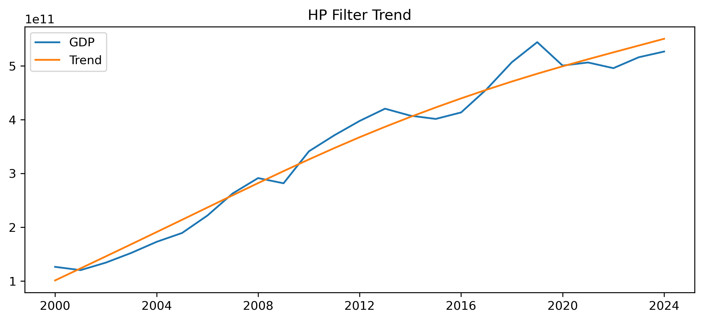

5.20 The Smoothing Parameter in the HP Filter¶

The HP filter uses a parameter:

\lambda

which controls smoothness.

Large $\lambda$ ¶

smoother trend,
less sensitivity to fluctuations.

Small $\lambda$ ¶

more flexible trend,
follows data more closely.

5.21 The Bias–Variance Trade-Off¶

Smoothing always involves compromise.

Too Little Smoothing¶

noisy estimates,
overreaction,
high variance.

Too Much Smoothing¶

important movements disappear,
turning points may be missed,
high bias.

5.22 Smoothing and Forecasting¶

Smoothing methods are often used as forecasting tools.

Examples include:

demand forecasting,
inventory management,
volatility estimation,
macroeconomic trend extraction.

5.23 Adjusted Prices and Trend Analysis¶

When working with financial prices, smoothing should usually be applied to:

Adjusted Close

rather than raw prices.

This becomes especially important in:

moving averages,
trend-following strategies,
backtesting.

5.24 Smoothing and Trading Indicators¶

Many popular trading indicators are essentially smoothing methods.

Examples include:

moving average crossover systems,
MACD,
Bollinger Bands.

5.25 Gretl Example: Moving Averages¶

Gretl provides simple tools for smoothing.

Step 1 — Open Data¶

Load a time series dataset.

Step 2 — Plot Series¶

Menu:

Variable → Time series plot

Step 3 — Add Moving Average¶

Menu:

Add → Moving average

Choose the window length.

[GRETL Screenshot Placeholder: Moving average dialog]

5.26 Gretl Example: HP Filter¶

Menu:

Variable → Filter → Hodrick-Prescott

Choose:

smoothing parameter,
trend extraction options.

[GRETL Screenshot Placeholder: HP filter output]

5.27 Common Mistakes¶

5.28 Looking Ahead¶

This chapter introduced methods for smoothing and trend estimation.

The next chapter studies how many popular trading indicators can be understood as filtering and smoothing techniques.

We will examine:

moving average crossover systems,
MACD,
RSI,
Bollinger Bands.

Key Takeaways¶

Concept Check¶

Basic¶

What is smoothing in time series analysis?
What is the goal of trend estimation?
What is the difference between signal and noise?

Intuition¶

Why do we smooth time series data before analyzing it?
What is the key idea behind exponential smoothing?
Why might recent observations be more informative than older ones?

Intermediate¶

What is the difference between:
- moving average
- exponential smoothing
- LOESS
What role do knots play in spline methods?
What is the purpose of the HP filter?

Finance Connection¶

What are adjusted prices?
Why are adjusted prices important in financial time series?

Challenge¶

What is the bias–variance trade-off?

What happens if a model is too smooth?
What happens if a model is too flexible?

Interpretation & Practice¶

A heavily smoothed series looks very stable.
- What is the advantage?
- What information might be lost?

A lightly smoothed series fluctuates a lot.
- What problem does this create?
- What type of noise might remain?

A LOESS curve follows the data closely.
- When is this useful?
- When might it lead to overfitting?

A spline model uses many knots.
- What happens to flexibility?
- What is the risk?

The HP filter separates a series into trend and cycle.
- What does the “cycle” represent?
- Why might this be useful in macroeconomics?

Finance Interpretation¶

A stock price shows a sudden drop due to a dividend payment.
- What happens to the raw price?
- Why do adjusted prices correct for this?

A trader uses a very smooth trend estimate.
- What type of strategy is this suited for?
- Why might it miss short-term signals?

Challenge¶

A model fits historical data very closely but performs poorly in forecasting.
- What problem is this?
- How is it related to the bias–variance trade-off?

Numerical Practice¶

Exponential Smoothing (Applied)¶

Consider the following data:

Week	Sales	Forecast
1	39	39
2	44	39
3	40	40
4	45	40
5	38	41
6	43	40.4
7	39	40.92

The smoothing parameter is:

\alpha = 0.2

Verify the forecast for Week 3 using:

F_{t+1} = \alpha A_t + (1-\alpha) F_t

Compute the forecast for Week 7.
Why does the forecast change more slowly than the actual data?
What would happen if:

α = 0.8 instead of 0.2?

Comparison Thinking¶

Suppose you apply:

moving average
exponential smoothing
LOESS

to the same dataset.

Which method is likely to be most flexible?
Which method is easiest to compute?
Which method is most responsive to recent changes?

Challenge¶

Suppose a model is extremely smooth and misses turning points.

What type of error is this?
How does this relate to bias?

Suppose a model follows every fluctuation in the data.

What type of problem is this?
How does this relate to variance?

Appendix 5A — Centered vs Trailing Moving Averages¶

A moving average may be:

trailing,
or centered.

Trailing Moving Average¶

Uses only past observations:

MA_t = \frac{1}{k} \sum_{i=0}^{k-1}x_{t-i}

This is common in forecasting and trading.

Centered Moving Average¶

Uses observations on both sides of $t$ .

Centered averages often produce smoother trend estimates but cannot be used in real-time forecasting.

Appendix 5B — Why “Exponential” Smoothing?¶

The name “exponential smoothing” comes from the fact that older observations receive exponentially decreasing weights.

Starting from:

\hat x_{t+1} = \alpha x_t + (1-\alpha)\hat x_t

we can substitute recursively:

\hat x_t = \alpha x_{t-1} + (1-\alpha)\hat x_{t-1}

Continuing this process yields:

\hat x_{t+1} = \alpha x_t + \alpha(1-\alpha)x_{t-1} + \alpha(1-\alpha)^2 x_{t-2} + \cdots

Appendix 5C — Why Smoothing Can Distort Turning Points¶

Heavy smoothing reduces noise but may delay detection of:

recessions,
market crashes,
trend reversals.

This creates an important trade-off in practical forecasting and trading systems.

Chapter 5 — Smoothing and Trend Estimation

Learning Objectives¶

5.1 Why Smooth Data?¶

5.2 Signal and Noise¶

Example¶

5.3 Moving Averages¶

Simple Moving Average¶

5.4 Example: 5-Day Moving Average¶

5.5 Moving Averages in Python¶

5.6 Choosing the Window Length¶

Small Window¶

Large Window¶

5.7 Moving Averages as Filters¶

5.8 Exponential Smoothing¶

Simple Exponential Smoothing¶

Alternative Form (Error-Correction View)¶

5.9 Interpreting the Smoothing Parameter¶

Large α\alphaα¶

Small α\alphaα¶

5.10 Exponential Smoothing in Python¶

5.11 Forecasting Interpretation¶

5.12 Holt’s Method¶

Holt Updating Equations¶

Level¶

Trend¶

5.13 Holt–Winters Method¶

5.14 Example: Seasonal Data¶

5.15 Local Smoothing: LOESS¶

5.16 LOESS Example in Python¶

5.17 Splines¶

Intuition¶

Why Not Use One Polynomial?¶

Role of Knots¶

Comparison with Other Methods¶

When Are Splines Useful?¶

5.18 The Hodrick–Prescott (HP) Filter¶

Decomposition¶

5.19 HP Filter Example¶

5.20 The Smoothing Parameter in the HP Filter¶

Large λ\lambdaλ¶

Small λ\lambdaλ¶

5.21 The Bias–Variance Trade-Off¶

Too Little Smoothing¶

Too Much Smoothing¶

5.22 Smoothing and Forecasting¶

5.23 Adjusted Prices and Trend Analysis¶

5.24 Smoothing and Trading Indicators¶

5.25 Gretl Example: Moving Averages¶

Step 1 — Open Data¶

Step 2 — Plot Series¶

Step 3 — Add Moving Average¶

5.26 Gretl Example: HP Filter¶

5.27 Common Mistakes¶

5.28 Looking Ahead¶

Key Takeaways¶

Concept Check¶

Basic¶

Intuition¶

Intermediate¶

Finance Connection¶

Challenge¶

Interpretation & Practice¶

Finance Interpretation¶

Challenge¶

Numerical Practice¶

Exponential Smoothing (Applied)¶

Comparison Thinking¶

Challenge¶

Appendix 5A — Centered vs Trailing Moving Averages¶

Trailing Moving Average¶

Centered Moving Average¶

Appendix 5B — Why “Exponential” Smoothing?¶

Appendix 5C — Why Smoothing Can Distort Turning Points¶

Large $\alpha$ ¶

Small $\alpha$ ¶

Large $\lambda$ ¶

Small $\lambda$ ¶