Chapter 22 — VAR Models - Applied Time Series

In earlier chapters, we studied models involving a single time series.

For example:

AR models explained persistence in one variable,
ARIMA models modeled trends and differencing,
ECM models described long-run equilibrium adjustment.

But many economic and financial variables evolve together.

Examples include:

inflation and interest rates,
GDP growth and unemployment,
exchange rates and inflation,
stock returns across markets.

Vector autoregression (VAR) models were developed precisely for this purpose.

This chapter introduces:

multivariate dynamics,
vector autoregressions,
lag selection,
impulse responses,
forecast error variance decompositions,
and VAR forecasting.

The emphasis is intuition-first and applications-oriented.

Learning Objectives¶

By the end of this chapter, you should be able to:

explain the intuition behind VAR models
distinguish univariate and multivariate models
estimate VAR models
interpret lagged interactions
understand impulse response functions
understand forecast error variance decomposition
select lag lengths
perform basic VAR forecasting
interpret VAR results economically

22.1 Why Multivariate Models?¶

Economic variables rarely move independently.

For example:

inflation influences interest rates,
interest rates influence investment,
investment influences GDP,
GDP influences unemployment.

A univariate AR model ignores these interactions.

VAR models attempt to capture them directly.

22.2 From AR Models to VAR Models¶

Recall the AR(1) model:

y_t = \alpha + \phi y_{t-1} + e_t

The current value depends on:

its own past,
plus a shock.

Extending to Multiple Variables¶

Suppose we have two variables:

inflation,
interest rate.

A VAR allows each variable to depend on:

its own lags,
and lags of the other variable.

22.3 A Simple VAR(1)¶

A two-variable VAR(1) may be written:

\pi_t = \alpha_1 + \beta_{11}\pi_{t-1} + \beta_{12}r_{t-1} + u_{1t}

r_t = \alpha_2 + \beta_{21}\pi_{t-1} + \beta_{22}r_{t-1} + u_{2t}

where:

$\pi_t$ = inflation,
$r_t$ = interest rate.

22.4 Why VAR Models Became Popular¶

VAR models became highly influential in macroeconomics and finance because they provide a flexible framework for studying dynamic interactions across variables.

Christopher Sims argued that many macroeconomic systems should be modeled jointly rather than through isolated single equations.

This contrasts with traditional regression models where some variables are treated as purely explanatory.

22.5 Endogenous and Exogenous Variables¶

In many regression models:

some variables are explanatory,
others are dependent.

VAR models are different.

This means:

inflation may affect interest rates,
but interest rates may also affect inflation.

The relationship is dynamic and simultaneous through time.

22.6 Reduced Form VARs¶

The most common VAR specification is the reduced form VAR.

A reduced form VAR expresses each variable as a function of lagged values of all variables in the system.

Example¶

Suppose we model:

inflation,
unemployment,
interest rate.

Then each equation includes:

lags of inflation,
lags of unemployment,
lags of interest rates.

22.7 VAR(p) Models¶

A VAR with multiple lags is written as VAR( $p$ ).

For example:

VAR(1),
VAR(2),
VAR(4).

General Form¶

Y_t = A_0 + A_1 Y_{t-1} + A_2 Y_{t-2} + \cdots + A_p Y_{t-p} + u_t

where:

$Y_t$ is a vector of variables,
$A_i$ are coefficient matrices,
$u_t$ is a vector of shocks.

As the number of variables and lags increases, estimation becomes more complex.

22.8 Stationarity in VAR Models¶

VAR models usually require stationary variables.

If variables are nonstationary:

spurious relationships may emerge,
inference becomes unreliable.

Common Approaches¶

If variables are nonstationary:

difference the data,
or use cointegration and VECM methods.

We studied these ideas in previous chapters.

22.9 Example: Inflation and Interest Rates¶

Suppose inflation rises persistently.

Central banks may respond by:

increasing interest rates.

But higher interest rates may later reduce:

inflation,
investment,
economic activity.

VAR models attempt to capture these dynamic feedback effects.

22.10 Estimating a VAR in Python¶

We now estimate a simple VAR model using inflation and interest rate data.

import yfinance as yf
import pandas as pd
import numpy as np

from statsmodels.tsa.api import VAR

# Download data
spy = yf.download(
    "SPY",
    start="2015-01-01",
    auto_adjust=False
)

# Compute returns
returns = 100 * np.log(
    spy["Adj Close"] /
    spy["Adj Close"].shift(1)
)

returns = returns.dropna()

# Create second variable
volatility = returns.rolling(20).std()

data = pd.concat(
    [returns, volatility],
    axis=1
)

data.columns = [
    "Returns",
    "Volatility"
]

data = data.dropna()

# Estimate VAR
model = VAR(data)

results = model.fit(2)

print(results.summary())

[*********************100%***********************]  1 of 1 completed
  Summary of Regression Results   
==================================
Model:                         VAR
Method:                        OLS
Date:           Thu, 30, Apr, 2026
Time:                     14:12:37
--------------------------------------------------------------------
No. of Equations:         2.00000    BIC:                   -4.95074
Nobs:                     2825.00    HQIC:                  -4.96419
Log likelihood:          -984.358    FPE:                 0.00693077
AIC:                     -4.97178    Det(Omega_mle):      0.00690631
--------------------------------------------------------------------
Results for equation Returns
================================================================================
                   coefficient       std. error           t-stat            prob
--------------------------------------------------------------------------------
const                 0.002458         0.037697            0.065           0.948
L1.Returns           -0.116849         0.018947           -6.167           0.000
L1.Volatility        -0.509801         0.271344           -1.879           0.060
L2.Returns            0.052044         0.018966            2.744           0.006
L2.Volatility         0.564860         0.271448            2.081           0.037
================================================================================

Results for equation Volatility
================================================================================
                   coefficient       std. error           t-stat            prob
--------------------------------------------------------------------------------
const                 0.009339         0.002575            3.627           0.000
L1.Returns           -0.008155         0.001294           -6.301           0.000
L1.Volatility         1.177278         0.018536           63.514           0.000
L2.Returns           -0.006887         0.001296           -5.316           0.000
L2.Volatility        -0.186537         0.018543          -10.060           0.000
================================================================================

Correlation matrix of residuals
               Returns  Volatility
Returns       1.000000   -0.121504
Volatility   -0.121504    1.000000

22.11 Choosing Lag Lengths¶

One important decision is:

How many lags should be included?

Too few lags:

omit important dynamics.

Too many lags:

waste degrees of freedom,
increase estimation noise.

22.12 Information Criteria¶

VAR lag lengths are often selected using:

AIC,
BIC,
HQIC.

Intuition¶

These criteria balance:

model fit,
and model complexity.

22.13 Lag Selection in Python¶

lag_selection = model.select_order(10)

print(lag_selection.summary())

 VAR Order Selection (* highlights the minimums)  
==================================================
       AIC         BIC         FPE         HQIC   
--------------------------------------------------
0      -0.7217     -0.7174      0.4859     -0.7201
1       -4.917      -4.904    0.007321      -4.912
2       -4.967      -4.946    0.006962      -4.960
3       -4.991      -4.962    0.006797      -4.981
4       -5.028      -4.990    0.006550      -5.015
5       -5.046      -4.999    0.006436      -5.029
6       -5.060      -5.006    0.006343      -5.041
7       -5.071      -5.007    0.006278      -5.048
8       -5.078      -5.006    0.006232      -5.052
9       -5.089     -5.009*    0.006166     -5.060*
10     -5.090*      -5.002   0.006155*      -5.058
--------------------------------------------------

In practice:

economic intuition,
diagnostics,
and forecasting performance

also matter.

22.14 Interpreting VAR Coefficients¶

Individual VAR coefficients are often difficult to interpret directly.

Why?

Because:

variables interact dynamically,
effects propagate over time,
feedback loops exist.

22.15 Impulse Response Functions (IRFs)¶

Impulse response functions are one of the most important VAR tools.

Example¶

Question:

What happens to inflation after an interest-rate shock?

IRFs attempt to answer this dynamically.

22.16 Intuition of Impulse Responses¶

Suppose interest rates unexpectedly rise today.

This shock may affect:

inflation,
output,
unemployment,
exchange rates.

And these effects may persist for many periods.

22.17 Impulse Responses in Python¶

import matplotlib.pyplot as plt

irf = results.irf(12)

irf.plot()

plt.savefig("figs/ch22/irf.png", dpi=300, bbox_inches="tight")
plt.close()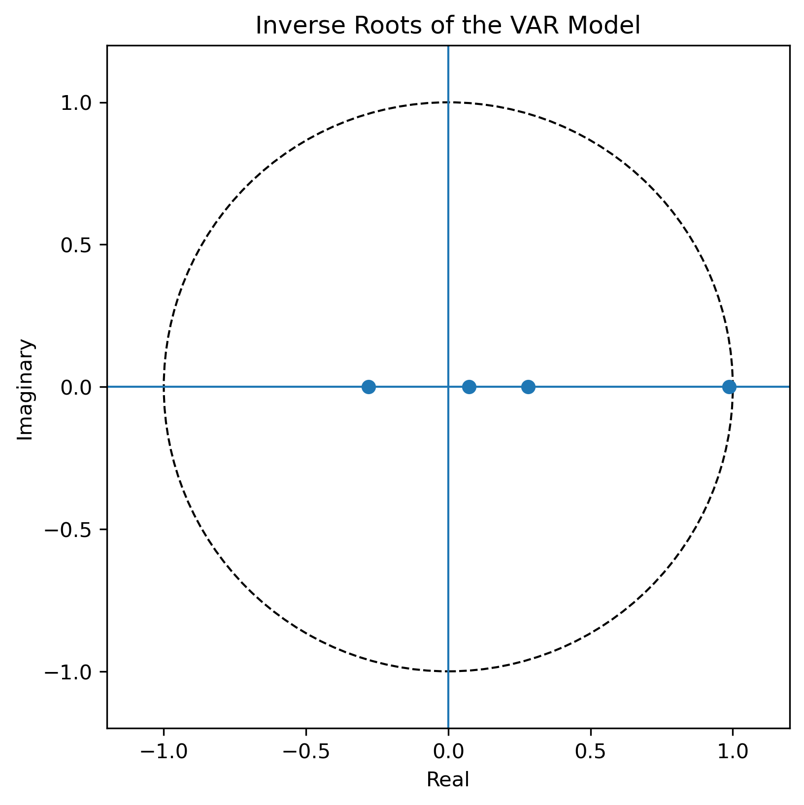   # replace with plt.show()

22.18 Forecast Error Variance Decomposition¶

Another important VAR tool is variance decomposition.

Example¶

How much of inflation uncertainty is explained by:

inflation shocks?
interest-rate shocks?

Variance decomposition helps answer this question.

22.19 Variance Decomposition in Python¶

fevd = results.fevd(12)

print(fevd.summary())

FEVD for Returns
       Returns  Volatility
0     1.000000    0.000000
1     0.998821    0.001179
2     0.998824    0.001176
3     0.998822    0.001178
4     0.998802    0.001198
5     0.998783    0.001217
6     0.998762    0.001238
7     0.998742    0.001258
8     0.998721    0.001279
9     0.998702    0.001298
10    0.998682    0.001318
11    0.998664    0.001336

FEVD for Volatility
       Returns  Volatility
0     0.014764    0.985236
1     0.034354    0.965646
2     0.055795    0.944205
3     0.067071    0.932929
4     0.074163    0.925837
5     0.078737    0.921263
6     0.081928    0.918072
7     0.084261    0.915739
8     0.086039    0.913961
9     0.087438    0.912562
10    0.088567    0.911433
11    0.089496    0.910504

22.20 Forecasting with VAR Models¶

VAR models are widely used for forecasting.

Because they incorporate:

multiple variables,
interactions,
and dynamic feedback,

they often outperform simple univariate models. :contentReference[oaicite:3]{index=3}

22.21 Example: VAR Forecasting¶

forecast = results.forecast(
    data.values[-2:],
    steps=10
)

forecast_df = pd.DataFrame(
    forecast,
    columns=data.columns
)

print(forecast_df)

    Returns  Volatility
0  0.113503    0.716344
1  0.041964    0.713565
2  0.044320    0.714654
3  0.038196    0.716929
4  0.038490    0.719438
5  0.038143    0.722006
6  0.038306    0.724563
7  0.038417    0.727095
8  0.038566    0.729598
9  0.038709    0.732069

22.22 Structural VARs (SVARs)¶

Basic VARs describe correlations and dynamics.

But economists are often interested in causality.

This leads to:

Structural VARs (SVARs)

22.23 Ordering and Identification¶

Impulse responses often depend on:

variable ordering,
identifying restrictions.

This is one of the major challenges in VAR analysis.

Example¶

Does monetary policy affect inflation immediately?

Or only with delays?

Different assumptions imply different structural interpretations.

22.24 Common Applications of VAR Models¶

VARs are widely used in:

macroeconomics,
monetary policy,
finance,
exchange-rate analysis,
business-cycle analysis.

Financial Applications¶

Examples include:

stock returns and volatility,
exchange rates and interest rates,
oil prices and inflation.

22.25 Gretl Example: Estimating a VAR¶

Gretl provides built-in tools for VAR estimation.

Step 1¶

Load multiple time series.

Example:

inflation,
interest rate,
GDP growth.

Step 2¶

Menu:

Model → Time Series → VAR

Step 3¶

Choose:

variables,
lag length,
deterministic terms.

[GRETL Screenshot Placeholder: VAR specification window]

22.26 Gretl Diagnostics¶

After estimation, GRETL provides:

residual diagnostics,
stability tests,
impulse responses,
variance decomposition.

[GRETL Screenshot Placeholder: VAR output]

22.27 Stability of VAR Models¶

A stable VAR produces impulse responses that eventually die out.

Unstable VARs may produce explosive dynamics.

22.28 Common Mistakes¶

22.29 Looking Ahead¶

VAR models provide a flexible framework for multivariate dynamics.

The next chapter introduces:

impulse response analysis in greater detail,
dynamic shock propagation,
and structural interpretation.

We will then extend these ideas to VECMs for cointegrated systems.

Key Takeaways¶

Concept Check¶

Basic¶

What is a VAR model?
How does a VAR differ from a univariate AR model?
What does it mean for all variables in a VAR to be endogenous?

Intuition¶

Why are multivariate models important in economics?
What type of interactions can VAR models capture?
Why is it unrealistic to model macroeconomic variables in isolation?

Structure¶

In a VAR(1), what variables appear on the right-hand side?
What does VAR( $p$ ) mean?
Why does the number of parameters increase quickly in VAR models?

Stationarity¶

Why is stationarity important in VAR models?
What are the consequences of estimating a VAR with nonstationary data?

Challenge¶

Why are VAR coefficients often difficult to interpret directly?

Interpretation & Practice¶

A VAR model shows that:

inflation depends on past interest rates
interest rates depend on past inflation
- What type of relationship does this suggest?

A VAR is estimated with too few lags.
- What might happen?

A VAR is estimated with too many lags.
- What problem might arise?

A model includes multiple variables with strong feedback.
- Why might a VAR be appropriate?

Lag Selection¶

AIC suggests 5 lags, BIC suggests 2 lags.
- Why might these differ?
- Which might you prefer?

Stationarity¶

Variables appear to be nonstationary.
- What should you do before estimating a VAR?

Numerical Practice¶

VAR Interpretation¶

Consider a VAR(1):

y_t = 0.5y_{t-1} + 0.3x_{t-1}

x_t = 0.2y_{t-1} + 0.6x_{t-1}

Does $y_t$ depend on past $x_t$ ?
Does $x_t$ depend on past $y_t$ ?

Lag Structure¶

Suppose you increase lag length from 1 to 4.

What happens to:
- number of parameters?
- estimation complexity?

Information Criteria¶

Suppose:

Lag	AIC	BIC
1	-4.5	-4.4
2	-4.8	-4.6
3	-4.9	-4.5

Which lag is chosen by AIC?
Which by BIC?

Interpretation¶

Suppose a variable responds strongly to its own lag.

What does this suggest?

Diagnostics¶

Residuals show autocorrelation.

What does this imply?
What should be done?

Challenge¶

Suppose a VAR includes 5 variables and 4 lags.

Why might this be problematic?

Interpretation¶

A coefficient on lagged inflation is positive and significant.
- What does this imply?
- Why might interpretation still be limited?

Challenge¶

Why should VAR results be interpreted using IRFs rather than raw coefficients?
Forecasting with VAR

Why might VAR models outperform univariate models?
What makes VAR forecasts dynamic?

Interpretation¶

Forecasts depend on previous forecasts.

Why?
Why might VAR forecasts still perform poorly in practice?

Appendix 22A — Why VARs Became Influential¶

VARs became highly influential because they offered a systematic way to model rich dynamics across multiple time series.

Earlier macroeconomic models often relied heavily on strong theoretical restrictions.

VARs instead emphasized:

empirical dynamics,
flexible interactions,
and forecasting performance.

This made them especially attractive for applied macroeconomics and finance.

Appendix 22B — Dynamic Forecasting¶

VAR forecasts are dynamic because future values depend recursively on previous forecasts.

For example:

\hat Y_{t+2}

depends partly on:

\hat Y_{t+1}

This recursive structure is one reason VAR forecasting can capture complex dynamic interactions across variables.