Chapter 25 — ARCH Models - Applied Time Series

In earlier chapters, we studied models for the mean of a time series.

For example:

AR models explained persistence,
ARIMA models explained trends and dynamics,
VAR models explained interactions across variables.

But financial time series often display another important feature.

Periods of calm are often followed by periods of turbulence.

Large shocks tend to cluster together.

ARCH models were developed precisely to model this behavior.

This chapter introduces:

conditional heteroskedasticity,
volatility clustering,
ARCH models,
ARCH testing,
and volatility forecasting.

The discussion emphasizes intuition and financial applications.

Learning Objectives¶

By the end of this chapter, you should be able to:

explain volatility clustering
distinguish homoskedasticity from heteroskedasticity
understand conditional variance
explain the intuition of ARCH models
estimate ARCH models
test for ARCH effects
interpret ARCH coefficients
visualize time-varying volatility

25.1 Volatility in Financial Markets¶

Financial returns rarely fluctuate with constant intensity.

Instead:

calm periods are followed by calm periods,
turbulent periods are followed by turbulent periods.

Large returns tend to cluster together.

Example: Stock Returns¶

During financial crises:

returns fluctuate dramatically,
uncertainty rises,
volatility increases sharply.

During stable periods:

returns fluctuate less,
volatility remains low.

This feature appears repeatedly in:

stock returns,
exchange rates,
cryptocurrency markets,
commodity prices.

25.2 Constant Variance vs Time-Varying Variance¶

Classical regression models often assume:

Var(e_t)=\sigma^2

where:

the variance is constant,
and does not change over time.

The Problem¶

Financial returns often violate this assumption.

Instead:

Var(e_t)

changes over time.

25.3 Conditional Variance¶

ARCH models focus on conditional variance rather than unconditional variance.

Intuition¶

If yesterday experienced a large shock, today may also be volatile.

Example¶

Suppose markets experienced a crash yesterday.

Would you expect volatility today to be:

unusually low?
or unusually high?

Most investors would expect volatility to remain elevated.

ARCH models formalize this intuition.

25.4 Volatility Clustering¶

Volatility clustering is one of the most important empirical features of financial returns.

A plot of returns often shows:

quiet periods,
followed by bursts of volatility.

The sign may change:

positive returns,
negative returns,

but the magnitude tends to persist.

25.5 A Simple ARCH(1) Model¶

The ARCH model was introduced by Robert Engle in 1982.

The simplest ARCH model is ARCH(1).

Mean Equation¶

Suppose returns follow:

r_t=\mu+e_t

where:

$\mu$ is the average return,
$e_t$ is the error term.

ARCH Variance Equation¶

The ARCH(1) variance equation is:

h_t = \alpha_0 + \alpha_1 e_{t-1}^2

where:

$h_t$ = conditional variance,
$e_{t-1}^2$ = previous squared shock,
$\alpha_0>0$ ,
$\alpha_1 \ge 0$ .

25.6 Intuition of ARCH¶

Suppose yesterday produced a large return shock:

e_{t-1}^2

Then the model predicts:

h_t

will increase.

Large shocks yesterday imply elevated volatility today.

25.7 Why Squared Errors?¶

Why do we square the errors?

Because volatility concerns magnitude rather than direction.

Both:

large positive shocks,
and large negative shocks

increase volatility.

Squaring removes the sign.

Example¶

Shock	Squared Shock
3	9
-3	9

Both imply high volatility.

25.8 ARCH as Volatility Memory¶

ARCH models create persistence in volatility.

Suppose:

yesterday experienced a large shock,
therefore today’s variance rises,
which increases the probability of large future shocks.

This creates volatility clustering naturally.

25.9 Simulating ARCH Data in Python¶

We now simulate an ARCH(1) process.

import numpy as np
import matplotlib.pyplot as plt

np.random.seed(123)

T = 500

alpha0 = 1
alpha1 = 0.8

e = np.zeros(T)
h = np.zeros(T)

z = np.random.normal(size=T)

h[0] = alpha0

for t in range(1, T):

    h[t] = alpha0 + alpha1 * e[t-1]**2

    e[t] = np.sqrt(h[t]) * z[t]

plt.figure(figsize=(10,4))

plt.plot(e)

plt.title("Simulated ARCH(1) Process")

plt.savefig("figs/ch25/arch.png", dpi=300, bbox_inches="tight")
plt.close()   # replace with plt.show()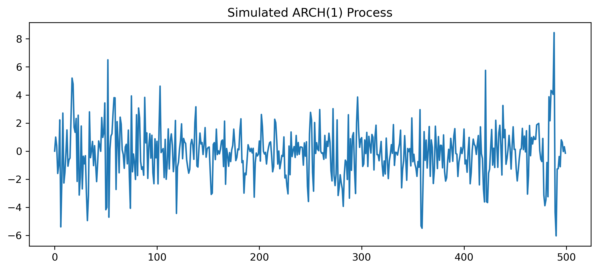

Even though the shocks are random, the variance evolves systematically through time.

25.10 ARCH Effects in Real Financial Data¶

ARCH effects are extremely common in:

stock returns,
exchange rates,
commodity prices,
cryptocurrency markets.

Financial returns often display:

volatility clustering,
fat tails,
changing risk over time.

Example from Financial Markets¶

[Figure Placeholder: Volatility clustering in stock returns]

25.11 Testing for ARCH Effects¶

Before estimating ARCH models, we usually test whether ARCH effects exist.

The test was developed by Engle.

Intuition Behind the ARCH Test¶

If volatility is constant:

e_t^2

should display little serial dependence.

But if volatility clusters, large squared residuals tend to follow large squared residuals.

Steps in the ARCH Test¶

Suppose we estimate:

r_t=\mu+e_t

using OLS.

Step 1 — Obtain Residuals¶

Compute residuals:

\hat e_t

Step 2 — Square the Residuals¶

Compute:

\hat e_t^2

Step 3 — Estimate Auxiliary Regression¶

Estimate:

\hat e_t^2 = \alpha_0 + \alpha_1 \hat e_{t-1}^2 + u_t

More generally, multiple lags may be included.

Step 4 — Compute the LM Statistic¶

where:

$T$ = sample size,
$R^2$ = coefficient of determination from the auxiliary regression.

Step 5 — Hypothesis Test¶

Under the null hypothesis:

H_0: \alpha_1=0

the statistic follows approximately:

\chi^2(q)

where:

$q$ = number of ARCH lags.

Interpreting the ARCH Test¶

Result	Interpretation
small p-value	evidence of ARCH
large p-value	little evidence of ARCH

Example of an ARCH Test¶

Suppose we obtain:

Statistic	Value
LM statistic	62.15
p-value	0.000

This implies volatility is not constant through time.

25.12 ARCH Estimation in Python¶

We now estimate an ARCH model using Python.

# !pip install arch

import yfinance as yf
import numpy as np
from arch import arch_model

sp500 = yf.download("^GSPC", start="2018-01-01", auto_adjust=False)

returns = 100 * np.log(
    sp500["Adj Close"] /
    sp500["Adj Close"].shift(1)
).dropna()

model = arch_model(
    returns,
    vol="ARCH",
    p=1
)

results = model.fit()

print(results.summary())

[*********************100%***********************]  1 of 1 completed
Iteration:      1,   Func. Count:      5,   Neg. LLF: 22080.30900905849
Iteration:      2,   Func. Count:     13,   Neg. LLF: 700493.8997438303
Iteration:      3,   Func. Count:     19,   Neg. LLF: 3163.8892644355155
Iteration:      4,   Func. Count:     25,   Neg. LLF: 3124.9447385811245
Iteration:      5,   Func. Count:     29,   Neg. LLF: 3124.944202980584
Iteration:      6,   Func. Count:     33,   Neg. LLF: 3124.9442004194407
Iteration:      7,   Func. Count:     36,   Neg. LLF: 3124.9442004194448
Optimization terminated successfully    (Exit mode 0)
            Current function value: 3124.9442004194407
            Iterations: 7
            Function evaluations: 36
            Gradient evaluations: 7
                      Constant Mean - ARCH Model Results                      
==============================================================================
Dep. Variable:                  ^GSPC   R-squared:                       0.000
Mean Model:             Constant Mean   Adj. R-squared:                  0.000
Vol Model:                       ARCH   Log-Likelihood:               -3124.94
Distribution:                  Normal   AIC:                           6255.89
Method:            Maximum Likelihood   BIC:                           6272.82
                                        No. Observations:                 2091
Date:                Thu, Apr 30 2026   Df Residuals:                     2090
Time:                        09:45:06   Df Model:                            1
                                Mean Model                                
==========================================================================
                 coef    std err          t      P>|t|    95.0% Conf. Int.
--------------------------------------------------------------------------
mu             0.1090  2.578e-02      4.226  2.380e-05 [5.843e-02,  0.159]
                            Volatility Model                            
========================================================================
                 coef    std err          t      P>|t|  95.0% Conf. Int.
------------------------------------------------------------------------
omega          0.7970  5.646e-02     14.115  3.052e-45 [  0.686,  0.908]
alpha[1]       0.4822  9.694e-02      4.974  6.562e-07 [  0.292,  0.672]
========================================================================

Covariance estimator: robust

25.13 Plotting Conditional Volatility¶

We now plot the estimated conditional volatility.

vol = results.conditional_volatility

vol.plot(figsize=(10,4))

plt.title("Estimated ARCH Volatility")

plt.savefig("figs/ch25/arch_vol.png", dpi=300, bbox_inches="tight")
plt.close()   # replace with plt.show()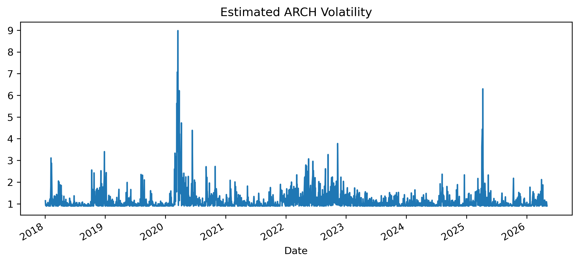

25.14 ARCH vs GARCH¶

ARCH models are useful but sometimes require many lag terms.

GARCH models solve this problem by including lagged variance terms.

We will study GARCH models in the next chapter.

ARCH(1)¶

h_t = \alpha_0 + \alpha_1 e_{t-1}^2

GARCH(1,1)¶

h_t = \omega + \alpha_1 e_{t-1}^2 + \beta_1 h_{t-1}

25.15 Gretl Example: Testing for ARCH¶

GRETL makes ARCH testing very straightforward.

Step 1 — Estimate a Regression Model¶

Menu:

Model → Ordinary Least Squares

Step 2 — Run ARCH Test¶

From the model window:

Tests → ARCH

Choose the number of ARCH lags.

[GRETL Screenshot Placeholder: ARCH test dialog]

Example Output¶

Null hypothesis: no ARCH effect is present

LM statistic = 62.15

p-value = 0.000

ARCH effects are present.

25.16 Gretl Example: Estimating ARCH¶

To estimate an ARCH(1) model:

Model → Time Series → GARCH

Then set:

GARCH order = 0
ARCH order = 1

[GRETL Screenshot Placeholder: ARCH estimation dialog]

25.17 Common Mistakes¶

25.18 Looking Ahead¶

ARCH models introduced the idea of modeling volatility dynamically.

However, pure ARCH models often require many lag terms.

The next chapter introduces:

GARCH models,
volatility persistence,
long-run variance,
and volatility forecasting.

Key Takeaways¶

Concept Check¶

Basic¶

What is volatility?
What is the difference between:
- mean
- variance
What does homoskedasticity mean?
What does heteroskedasticity mean?

Intuition¶

What is volatility clustering?
Why do financial returns often display clustering in volatility?
Why do large shocks tend to be followed by large shocks?
Why is volatility easier to “see” than to model?

ARCH Structure¶

What is the key idea behind an ARCH model?
What does the equation

h_t = \alpha_0 + \alpha_1 e_{t-1}^2

represent?

Why are squared residuals used?
Suppose volatility spikes after a large shock.

What does this suggest?

Interpretation¶

What does a large value of $\alpha_1$ imply?
What does it mean if $\alpha_1 = 0$ ?

Challenge¶

Can volatility be predictable even if returns are not?
You analyze stock returns and find:

no autocorrelation in returns
strong autocorrelation in squared returns

What does this imply?
Why might an ARCH model be appropriate?

Interpretation & Practice¶

A return series shows:

periods of calm
followed by periods of turbulence
- What does this suggest?

Residuals show no autocorrelation, but squared residuals do.
- What does this imply?
A model assumes constant variance, but volatility clearly changes.
- What problem arises?
An ARCH model is estimated and $\alpha_1$ is significant.
- What does this indicate?

Economic Interpretation¶

A financial crisis leads to large return shocks.
- What does the ARCH model predict for future volatility?
A period of calm persists.
- What does the model predict?

Challenge¶

Why might volatility clustering be important for risk management?

Numerical Practice¶

Squared Shocks¶

Suppose shocks are:

2, -3, 1

Compute squared shocks.

ARCH Equation¶

Suppose:

h_t = 1 + 0.5 e_{t-1}^2

and:

e_{t-1} = 2

Compute $h_t$ .

Suppose:

e_{t-1} = -2

Compute $h_t$ again.
What do you observe?

Interpretation¶

Suppose $\alpha_1 = 0.8$ .

What does this imply about volatility persistence?

Suppose $\alpha_1 = 0.1$ .

How does this differ?

Stability¶

What happens if $\alpha_1 \ge 1$ ?

Challenge¶

Suppose:

small shocks yesterday
small variance today
What does the model predict for tomorrow?

ARCH Testing¶

What is the purpose of the ARCH LM test?
What is the null hypothesis?

Interpretation¶

Suppose:

LM statistic = 45
p-value = 0.000
What is your conclusion?

Suppose:

p-value = 0.40
What does this imply?

Conceptual¶

Why does the ARCH test use squared residuals?

Challenge¶

Why is autocorrelation in squared residuals important?

Graph Interpretation¶

Volatility Clustering¶

Consider the following simulated return series:

import numpy as np
import matplotlib.pyplot as plt

np.random.seed(123)

T = 300
alpha0 = 1
alpha1 = 0.8

e = np.zeros(T)
h = np.zeros(T)

z = np.random.normal(size=T)

h[0] = alpha0

for t in range(1, T):
    h[t] = alpha0 + alpha1 * e[t-1]**2
    e[t] = np.sqrt(h[t]) * z[t]

plt.figure(figsize=(10,4))
plt.plot(e)
plt.title("Simulated ARCH(1) Returns")
plt.axhline(0, linestyle='--', linewidth=1)
plt.tight_layout()

plt.savefig("figs/ch25/rtn_Q.png", dpi=300, bbox_inches="tight")
plt.close()   # replace with plt.show()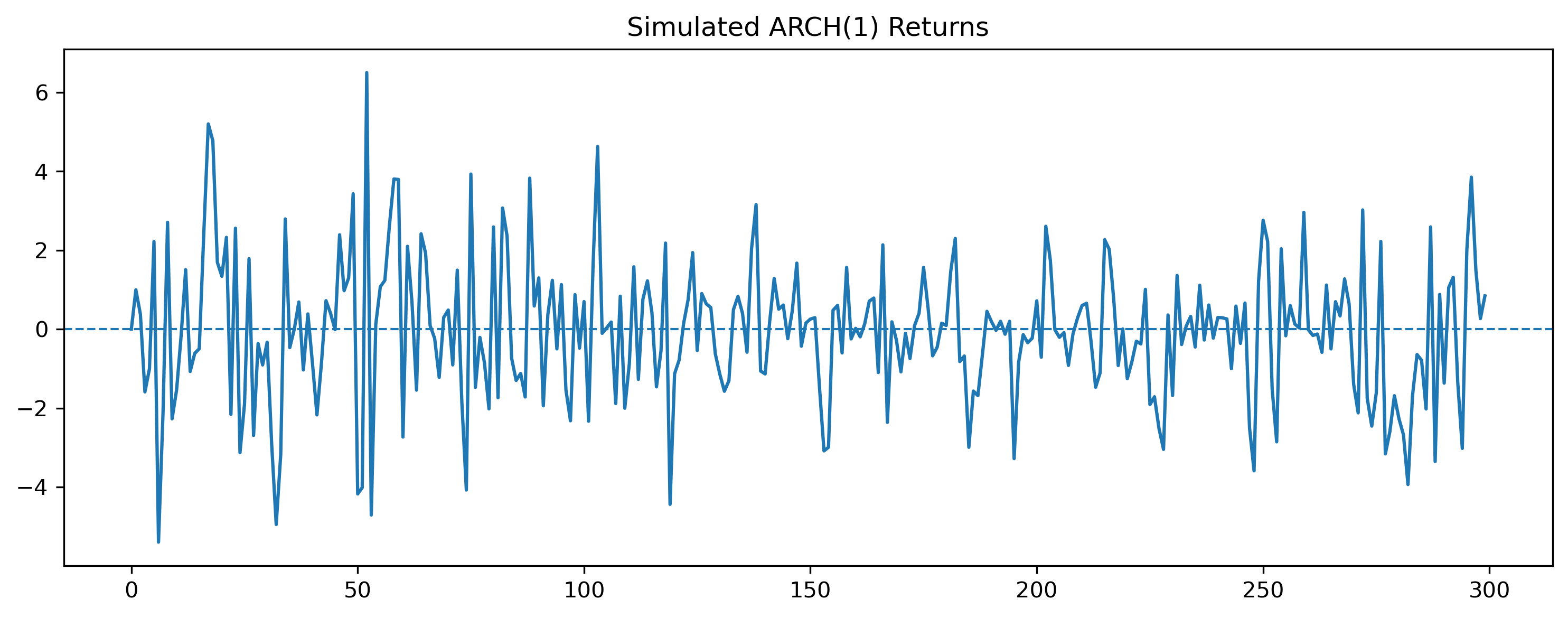

What feature of financial data does this illustrate?
Identify periods of:
- high volatility
- low volatility
Why is this inconsistent with constant variance?
Why might a standard regression model fail to capture this behavior?

Appendix 25A — ARCH(1) Stability Condition¶

For the ARCH(1) model:

h_t = \alpha_0 + \alpha_1 e_{t-1}^2

the parameter restrictions are:

\alpha_0>0

and:

0 \le \alpha_1 < 1

The condition:

\alpha_1<1

ensures the variance process remains stable.

If:

\alpha_1 \ge 1

volatility may become explosive.

Appendix 25B — Why Financial Returns Often Display Fat Tails¶

ARCH processes naturally generate:

clusters of volatility,
periods of calm,
and occasional extreme observations.

Even if the underlying shocks are normal, the resulting returns may appear fat-tailed.

This is one reason ARCH and GARCH models became so influential in finance.