Chapter 13 — ARMA Models
In the previous chapters, we studied:
autoregressive (AR) models
moving average (MA) models
Each captures a different type of dependence:
AR models depend on past values
MA models depend on past shocks
In practice, many time series exhibit both types simultaneously.
This motivates the ARMA model.
Learning Objectives
By the end of this chapter, you should be able to:
understand the motivation behind ARMA models
define ARMA() processes
interpret AR and MA components jointly
understand stationarity and invertibility
interpret ACF and PACF behavior
estimate ARMA models
perform diagnostics
13.1 Why Combine AR and MA?
AR models:
capture persistence
MA models:
capture temporary shock propagation
But real-world data often show both.
13.2 The ARMA(1,1) Model
Interpretation
The present depends on:
past values (persistence)
current shocks
past shocks
13.3 Simulation
import numpy as np
import matplotlib.pyplot as plt

np.random.seed(123)

n = 400
phi = 0.7
theta = 0.5

w = np.random.normal(size=n)
x = np.zeros(n)

for t in range(1,n):
    x[t] = phi*x[t-1] + w[t] + theta*w[t-1]

plt.figure(figsize=(10,4))
plt.plot(x, lw=1)
plt.title(r"ARMA(1,1): $\phi=0.7,\ \theta=0.5$")

plt.savefig("figs/ch13/arma11.png", dpi=300, bbox_inches="tight")
plt.close()   # replace with plt.show()
13.4 Mean
Without a constant:
13.5 Stationarity and Invertibility
ARMA requires:
Stationarity (AR part)
Invertibility (MA part)
13.6 Backshift Form
13.7 Infinite MA Representation
13.8 Infinite AR Representation
13.9 ACF and PACF Behavior
Why?
13.10 Simulated ACF/PACF
from statsmodels.graphics.tsaplots import plot_acf, plot_pacf

fig, ax = plt.subplots(2,1, figsize=(8,6))

plot_acf(x, lags=30, ax=ax[0])
plot_pacf(x, lags=30, method='ywm', ax=ax[1])

plt.tight_layout()

plt.savefig("figs/ch13/arma11_acf_pacf.png", dpi=300, bbox_inches="tight")
plt.close()   # replace with plt.show()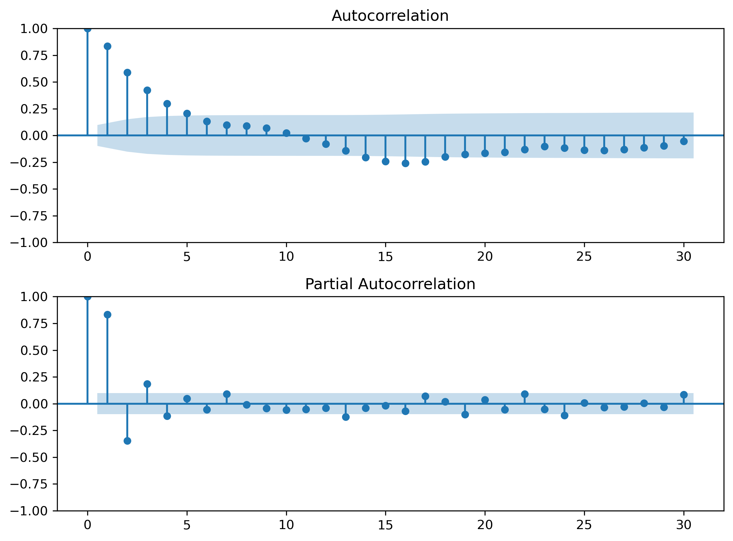
13.11 AR vs MA vs ARMA
| Model | ACF | PACF |
|---|---|---|
| AR | tails off | cuts off |
| MA | cuts off | tails off |
| ARMA | tails off | tails off |
13.12 Identification in Practice
Steps:
visualize data
ensure stationarity
inspect ACF/PACF
estimate candidates
check diagnostics
compare models
13.13 Estimation
import statsmodels.api as sm

model = sm.tsa.ARIMA(x, order=(1,0,1))
res = model.fit()

print(res.summary())
SARIMAX Results
==============================================================================
Dep. Variable: y No. Observations: 400
Model: ARIMA(1, 0, 1) Log Likelihood -564.412
Date: Mon, 04 May 2026 AIC 1136.824
Time: 22:05:59 BIC 1152.790
Sample: 0 HQIC 1143.147
- 400
Covariance Type: opg
==============================================================================
coef std err z P>|z| [0.025 0.975]
------------------------------------------------------------------------------
const -0.2646 0.248 -1.068 0.286 -0.750 0.221
ar.L1 0.6901 0.044 15.840 0.000 0.605 0.775
ma.L1 0.5423 0.049 11.081 0.000 0.446 0.638
sigma2 0.9803 0.069 14.148 0.000 0.845 1.116
===================================================================================
Ljung-Box (L1) (Q): 0.07 Jarque-Bera (JB): 0.11
Prob(Q): 0.80 Prob(JB): 0.95
Heteroskedasticity (H): 0.70 Skew: 0.04
Prob(H) (two-sided): 0.04 Kurtosis: 3.01
===================================================================================13.14 Diagnostics
from statsmodels.stats.diagnostic import acorr_ljungbox

acorr_ljungbox(res.resid, lags=[10,20], return_df=True)
| | lb_stat | lb_pvalue |
|---------|------------|-----------|
| 10 | 4.229114 | 0.936420 |
| 20 | 25.470103 | 0.184034 |
13.15 Information Criteria
13.16 Applications
ARMA models are used for:
inflation
GDP growth
exchange rates
interest rates
demand forecasting
13.17 Common Mistakes
13.18 Looking Ahead
Next:
Key Takeaways
Concept Check
Basic
What is an ARMA model?
What are the two components of an ARMA model?
What does the AR component capture?
What does the MA component capture?
Intuition
Why do many real-world time series require both AR and MA components?
How does an ARMA model differ from a pure AR or pure MA model?
What happens when both persistence and short-term shocks influence a series?
Intermediate
What are the stationarity and invertibility conditions for an ARMA(1,1) model?
Why must both conditions hold?
What is the backshift representation of an ARMA model?
ACF & PACF
What pattern does the ACF of an ARMA model exhibit?
What pattern does the PACF of an ARMA model exhibit?
Why do ARMA models not show sharp cutoffs in ACF or PACF?
Interpretation
Why is model identification more difficult for ARMA models than for AR or MA models?
Why should ACF and PACF be used cautiously in ARMA identification?
Challenge
Suppose a time series exhibits both:
strong persistence
short-lived shock effects
Why is ARMA a natural model?
Interpretation & Practice
A time series shows:
gradual decay in ACF
gradual decay in PACF
What type of model might this suggest?
Why?
ACF and PACF do not show clear cutoff patterns.
Why might this happen?
What modeling approach would you take?
A series appears smoother than pure AR but still persistent.
What might this indicate?
A model captures persistence but leaves short-term fluctuations unexplained.
What component might be missing?
A model captures shocks well but fails to capture persistence.
What component might be missing?
Finance Interpretation
A financial time series shows:
short-term reaction to news
longer-term persistence
Why might ARMA be appropriate?
A return series appears unpredictable but slightly autocorrelated.
What type of structure might exist?
Diagnostics
After estimating an ARMA model, residuals still show autocorrelation.
What does this imply?
What should you do next?
Challenge
Two ARMA models fit equally well visually.
How would you choose between them?
Numerical Practice
ARMA Construction
Consider:
with:
Compute
Comparing Models
Compare:
AR(1):
MA(1):
Which shows longer persistence?
Which shows finite shock effects?
ACF Interpretation
Suppose you observe:
ACF decays gradually
PACF also decays gradually
What model class is suggested?
Identification
You observe:
ACF does not cut off
PACF does not cut off
Why is ARMA a candidate model?
Estimation Output
Suppose:
Is the series persistent?
Are shocks temporary or long-lasting?
What does this imply about dynamics?
Diagnostics
Suppose residuals show:
significant autocorrelation
What does this imply?
What should be done?
Model Selection
Suppose two models produce:
Model A: lower AIC
Model B: lower BIC
What does this suggest?
How would you decide?
Challenge
Suppose an ARMA model fits the data well but performs poorly in forecasting.
What might be the issue?
Why is validation important?
Suppose is close to 1 and is large.
What type of behavior would you expect?
Why might this resemble a near-nonstationary process?
A time series shows:
moderate persistence
small but noticeable short-term fluctuations
no clear ACF cutoff
What model would you try first? Why?
Appendix 13A — Additional Insight
A.1 Why ACF Tails Off
AR component generates:
gradual decay in correlations
MA component adds:
short-term structure
Combined → no cutoff
A.2 Infinite Representations
ARMA can be expressed as:
infinite MA (if stationary)
infinite AR (if invertible)