Chapter 18 — Dynamic Regression and ARDL Models
In the previous chapter, we saw that regressions involving nonstationary variables can produce spurious results.
One common response was to difference the data:
At first glance, this may look like a technical fix. But it is more than that.
This chapter introduces dynamic regression models more generally. These models allow us to study how relationships unfold over time.
Learning Objectives
By the end of this chapter, you should be able to:
explain what a dynamic regression model is
distinguish static and dynamic models
understand distributed lag models
understand autoregressive distributed lag (ARDL) models
interpret short-run and long-run effects
diagnose residual autocorrelation
explain why differencing may remove long-run information
understand how dynamic models lead naturally to cointegration and ECM
18.1 From Spurious Regression to Dynamics
Recall the differenced regression:
This model no longer explains the level of using the level of . Instead, it explains how changes in one variable are related to changes in another.
For example:
how changes in income affect changes in consumption
how changes in interest rates affect changes in investment
how changes in exchange rates affect changes in exports
This is already a dynamic way of thinking.
18.2 What Is a Dynamic Model?
A dynamic model allows current outcomes to depend on time-related information, such as:
past values of the dependent variable
past values of explanatory variables
current and past changes
past shocks
Static vs Dynamic Models
A static model is:
This says that responds immediately to .
A dynamic model might be:
Here, depends not only on , but also on its own past value.
18.3 Why Dynamics Matter
Many economic relationships do not adjust instantly.
For example:
consumption may respond gradually to income
investment may respond slowly to interest rates
prices may adjust with delays
money demand may depend on past money balances
This makes them especially useful in economics, finance, and business forecasting.
18.4 Distributed Lag Models
A natural way to introduce dynamics is to include current and past values of an explanatory variable.
A simple distributed lag model is:
Here:
measures the immediate effect of
measures the effect of last period’s
measures the effect from two periods ago
Short-Run and Cumulative Effects
In the distributed lag model:
the short-run effect is:
The cumulative effect over three periods is:
18.5 Autoregressive Distributed Lag Models
We now combine two ideas:
lagged dependent variables
lagged explanatory variables
This gives the autoregressive distributed lag model, or ARDL.
where:
is the number of lags of
is the number of lags of
captures persistence in
captures current and lagged effects of
18.6 Interpreting an ARDL Model
Consider a simple ARDL(1,1):
The coefficients have different roles:
→ immediate effect
→ delayed effect
→ persistence in
18.7 Short-Run and Long-Run Effects
Dynamic models distinguish between:
short-run responses
long-run cumulative effects
For the ARDL(1,1):
the immediate short-run effect is:
If the system is stable, the long-run multiplier is:
More generally:
18.8 Dynamic Interpretation
Consider an increase in interest rates.
Its effect on output may not be immediate:
firms may delay investment decisions
households may adjust spending gradually
banks may adjust lending conditions over time
A dynamic model allows this adjustment path to be represented explicitly.
18.9 Differencing as a Restricted Dynamic Model
Recall from Chapter 17:
This can be viewed as a restricted dynamic model:
no lagged levels
no persistence term
no long-run structure
This is useful for avoiding spurious regression, but it may discard economically meaningful long-run information.
18.10 Why Differencing Is Not Enough
While differencing often solves the spurious regression problem, it comes at a cost.
Differencing may remove:
long-run relationships
equilibrium behavior
information about levels
gradual adjustment mechanisms
This motivates cointegration and the error correction model.
18.11 Looking Ahead: ECM
Dynamic models (ARDL) attempt to bridge this gap by modeling:
short-run changes
long-run relationships
in a unified framework.
If two variables share a long-run equilibrium relationship, we may want to model both:
short-run changes
adjustment back toward the long-run relationship
This leads to the Error Correction Model (ECM):
We return to this idea in later chapters.
18.12 Gretl Example: ARDL Model
We now estimate a simple ARDL model using the denmark dataset in GRETL.
Step 1: Load the Data
Menu
File → Open data → Sample file...
Select the denmark data from the GRETL database.
The variables include:
LRM     log of real money supply, M2
LRY     log of real income
IBO     bond rate
IDE     bank deposit rate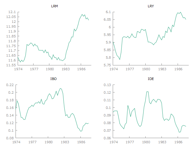
Figure 1:Denmark macroeconomic data
Step 2: Estimate ARDL(1,1)
We estimate:
Menu
Model → Ordinary Least Squares
Dependent variable:
LRMRegressors:
LRM(-1) LRY LRY(-1)
To create lags, click the lags... icon in the model specification window.
Command
ols LRM const LRM(-1) LRY LRY(-1)Example output:
Model 1: OLS, using observations 1974:2-1987:3 (T = 54)
Dependent variable: LRM

             coefficient   std. error   t-ratio    p-value
  ---------------------------------------------------------
  const        0.125046    0.342856      0.3647   0.7169
  LRM_1        1.00090     0.0580381    17.25     1.09e-022 ***
  LRY          0.630431    0.173817      3.627    0.0007    ***
  LRY_1       −0.652328    0.170176     −3.833    0.0004    ***

Mean dependent var   11.75666   S.D. dependent var   0.152858
Sum squared resid    0.044114   S.E. of regression   0.029703
R-squared            0.964377   Adjusted R-squared   0.962240
F(3, 50)             451.2022   P-value(F)           3.49e-36
Log-likelihood       115.3464   Akaike criterion    −222.6929
Schwarz criterion   −214.7370   Hannan-Quinn        −219.6246
rho                 −0.186568   Durbin's h          −1.515760
This can be written as:
18.13 Diagnosing ARDL Models
After estimating an ARDL model, we need to check whether the model has captured the relevant dynamics.
If residuals still contain autocorrelation, the model is missing some dynamic structure.
What Do We Mean by White Noise Residuals?
Residuals should show:
mean near zero
roughly constant variance
no autocorrelation
Step 1: Plot Residuals
Menu
Graph → Time series plot
Select residuals, such as uhat.
You can also right click on the residual variable and select Time series plot.
Command
gnuplot uhat --time-series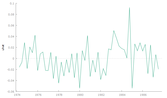
Figure 2:Residual plot
Step 2: Residual Correlogram
Menu
Select uhat.
Variable → Correlogram
You can also right click on uhat and select Correlogram.
Command
corrgm uhat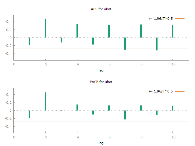
Figure 3:Correlogram of residuals
Step 3: Formal Test for Serial Correlation
In the model window:
Tests → Autocorrelation
GRETL reports tests such as the Breusch–Godfrey test and Ljung–Box Q test.
Example output:
Breusch-Godfrey test for autocorrelation up to order 4
OLS, using observations 1974:2-1987:3 (T = 54)
Dependent variable: uhat

             coefficient   std. error   t-ratio    p-value
  --------------------------------------------------------
  const       0.342059     0.336486      1.017     0.3147
  LRY        −0.00513435   0.162471     −0.03160   0.9749
  LRY_1       0.0773596    0.173429      0.4461    0.6576
  LRM_1      −0.0657127    0.0631492    −1.041     0.3035
  uhat_1     −0.0607536    0.158039     −0.3844    0.7024
  uhat_2      0.427085     0.147320      2.899     0.0057  ***
  uhat_3      0.110868     0.162276      0.6832    0.4979
  uhat_4      0.240594     0.160901      1.495     0.1417

  Unadjusted R-squared = 0.283633

Test statistic: LMF = 4.553230,
with p-value = P(F(4,46) > 4.55323) = 0.0035

Alternative statistic: TR^2 = 15.316197,
with p-value = P(Chi-square(4) > 15.3162) = 0.00409

Ljung-Box Q' = 23.0858,
with p-value = P(Chi-square(4) > 23.0858) = 0.000122What If Residuals Are Not White Noise?
If residuals show autocorrelation, possible responses include:
add more lags of
add more lags of
reconsider the model specification
check whether variables are nonstationary
consider cointegration or ECM if levels matter
Important Distinction
18.14 Practical Checklist
18.15 Common Mistakes
18.16 Looking Ahead
Dynamic models help us understand how variables adjust over time.
But they do not fully resolve the issue of nonstationarity.
Is it possible to retain long-run information while avoiding spurious regression?
Yes — if a particular combination of nonstationary variables is stationary.
This concept is called cointegration, which we study later.
Key Takeaways
Concept Check
Basic
What is a dynamic regression model?
What is the difference between a static and a dynamic model?
What is a distributed lag model?
Intuition
Why do many economic relationships adjust gradually rather than instantly?
What does it mean for effects to “unfold over time”?
Why is including lagged variables important?
ARDL Models
What are the two key components of an ARDL model?
What does the lagged dependent variable capture?
What do lagged explanatory variables capture?
Short-Run vs Long-Run
What is the short-run effect in a distributed lag model?
What is the long-run multiplier?
Why are these two effects different?
Diagnostics
What should residuals look like in a well-specified dynamic model?
Why is residual autocorrelation a problem?
Challenge
Why is differencing alone not sufficient for economic modeling?
Interpretation & Practice
A static model shows poor fit, but a dynamic model fits well.
What does this suggest?
A model includes lagged dependent variables.
What type of behavior is being captured?
Residuals show strong autocorrelation.
What does this imply?
What should you do?
A model shows strong short-run effects but weak long-run effects.
What might this indicate?
A model shows large long-run multiplier.
What does this imply about persistence?
Trade-Off Interpretation
Differencing removes long-run relationships.
Why is this a problem?
A levels regression shows strong relationship but residuals are nonstationary.
What does this imply?
Challenge
Why might ARDL be preferred over simple differencing?
Numerical Practice
Distributed Lag
Suppose:
What is the immediate effect?
What is the cumulative effect?
ARDL(1,1)
Suppose:
What is the short-run effect?
Compute the long-run multiplier.
Interpretation
If , what does this imply about adjustment speed?
Diagnostics
Residual correlogram shows significant spikes.
What does this imply?
Model Improvement
What are two ways to improve a poorly specified ARDL model?
Challenge
Suppose:
levels regression → spurious
differenced regression → no relationship
What should you try next?
Appendix 18A — Dynamic Models and Long-Run Effects
This appendix shows how long-run effects arise from a simple ARDL model.
A.1 A Simple ARDL(1,1)
Consider:
A.2 Steady-State Long-Run Equilibrium
In the long run, suppose:
Substitute these into the ARDL(1,1) model:
So:
Rearranging:
Therefore:
A.3 Stability Condition
For the long-run expression to be meaningful, the process must be dynamically stable.
For ARDL(1,1), this requires:
A.4 Dynamic Adjustment
Start again from:
Subtract from both sides:
Since:
we can write:
This expression begins to reveal the link between ARDL and ECM.
A.5 Link to ECM
An ECM has the form:
The ECM representation makes this separation explicit.
Appendix 18B — ARDL Bounds Test for Cointegration
The ARDL framework can also be used to test for long-run relationships between variables.
This approach is known as the ARDL bounds testing procedure (Pesaran et al.).
B.1 Motivation
Recall the key problem:
Levels regression → may be spurious
Differenced regression → loses long-run information
B.2 From ARDL to Error Correction Form
Consider an ARDL(1,1):
This can be rewritten as:
where:
B.3 The Bounds Test
We test:
No long-run relationshipagainst:
At least one is non-zero → long-run relationship existsB.4 Decision Rule
The test uses an F-statistic.
Compare it with two bounds:
Lower bound → assumes variables are stationary
Upper bound → assumes variables are nonstationary
B.5 Why This Is Useful
B.6 Intuition
B.7 Link to ECM
If cointegration is confirmed, we can write:
B.8 Important Caution
B.9 Looking Ahead
We will study cointegration formally in Chapter 20.