Chapter 23 — Impulse Response Functions

In the previous chapter, we introduced VAR models as systems of interacting time series.

VAR models allow:

multiple variables,
dynamic feedback,
and recursive interactions

to be modeled jointly.

But VAR coefficient tables are often difficult to interpret directly.

Suppose we estimate a VAR involving:

stock returns,
volatility,
interest rates,
or inflation.

A natural question immediately arises:

Impulse response functions (IRFs) were developed precisely to answer such questions.

IRFs trace:

how shocks propagate,
how long effects persist,
and how systems gradually adjust through time.

This chapter introduces:

dynamic shock propagation,
impulse response functions,
orthogonalization,
identification,
confidence intervals,
and forecast error variance decomposition (FEVD).

The emphasis remains intuition-first and applications-oriented.

Learning Objectives¶

By the end of this chapter, you should be able to:

explain the intuition behind impulse response functions
interpret dynamic responses to shocks
distinguish contemporaneous and lagged effects
understand orthogonalized shocks
interpret confidence bands
generate IRFs in Python and GRETL
understand identification issues in VAR analysis
interpret IRFs economically

23.1 Why Impulse Responses Matter¶

Economic systems are dynamic.

A shock today may influence variables:

immediately,
gradually,
or persistently.

For example:

a monetary tightening may reduce inflation only slowly,
an oil-price shock may affect output for many quarters,
a financial crisis may generate persistent volatility.

23.2 What Is an Impulse Response Function?¶

The response is tracked period by period.

Example¶

Suppose interest rates suddenly increase unexpectedly.

We may ask:

How does inflation respond?
How long do effects persist?
Do effects eventually disappear?

IRFs attempt to answer these questions visually and dynamically.

23.3 Why VAR Coefficients Are Difficult to Interpret¶

In univariate models, coefficients are often interpreted directly.

VAR systems are different.

Because variables interact dynamically:

effects propagate across variables,
responses accumulate through time,
and feedback loops emerge.

A shock today may influence:

tomorrow,
next week,
or many future periods.

This is why IRFs became one of the central tools of modern macroeconomics and finance.

23.4 Intuition: Dropping a Stone into Water¶

A useful analogy is:

Dropping a stone into water.

The initial splash creates waves.

The waves then:

spread,
interact,
and gradually disappear.

Economic shocks behave similarly.

23.5 Impulse Responses in a VAR¶

Consider a VAR involving:

inflation,
interest rate.

Suppose an unexpected interest-rate shock occurs today.

The VAR traces:

inflation tomorrow,
inflation next month,
inflation next year,
and so on.

Dynamic Feedback¶

Because variables interact:

inflation affects interest rates,
interest rates affect inflation,
and responses feed back through time.

This creates rich dynamic behavior.

Example¶

Suppose central banks unexpectedly raise interest rates.

Possible dynamic effects include:

Period	Possible Effect
immediate	borrowing becomes more expensive
short run	investment falls
medium run	output slows
longer run	inflation declines

23.6 Reading Impulse Response Functions¶

Impulse response functions contain several types of economic information.

When reading an IRF, economists often focus on:

direction,
timing,
persistence,
and stability.

Direction¶

Does the response move:

upward,
downward,
or change sign through time?

Timing¶

Does the response occur:

immediately,
gradually,
or with delay?

Persistence¶

Do effects disappear quickly?

Or do they remain for many periods?

Stability¶

Does the response eventually return toward zero?

Oscillation¶

Some responses:

overshoot,
fluctuate,
and oscillate before stabilizing.

This often reflects rich dynamic feedback within the system.

Positive and Negative Responses¶

Impulse responses may be:

positive,
negative,
or mixed over time.

For example:

a monetary tightening may reduce inflation,
an oil-price shock may initially raise inflation,
stock markets may react positively or negatively depending on expectations.

23.7 Common Shapes of Impulse Responses¶

Impulse responses may display several common dynamic patterns.

Understanding these patterns helps economists interpret dynamic systems more effectively.

Rapidly Decaying Response¶

Some shocks disappear quickly.

This suggests:

weak persistence,
fast adjustment,
and strong system stability.

import numpy as np
import matplotlib.pyplot as plt

h = np.arange(15)

irf = np.exp(-0.8*h)

plt.figure(figsize=(7,4))

plt.plot(h, irf, marker="o")

plt.axhline(0, linestyle="--", linewidth=1)

plt.title("Rapidly Decaying Impulse Response")
plt.xlabel("Horizon")
plt.ylabel("Response")

plt.tight_layout()

plt.savefig("figs/ch23/rapid_decay.png",
            dpi=300,
            bbox_inches="tight")

plt.close()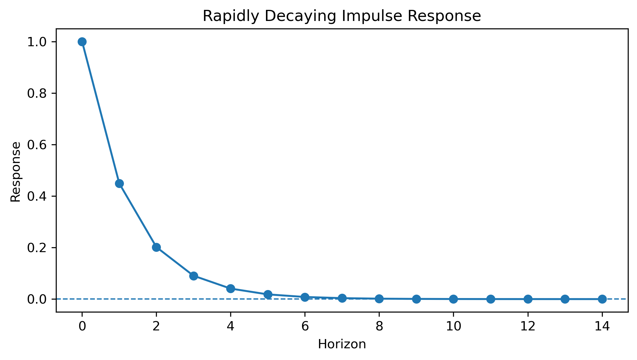

Persistent Response¶

Some shocks decay only gradually.

This suggests:

strong persistence,
long memory,
or slow adjustment dynamics.

h = np.arange(20)

irf = 0.95**h

plt.figure(figsize=(7,4))

plt.plot(h, irf, marker="o")

plt.axhline(0, linestyle="--", linewidth=1)

plt.title("Persistent Impulse Response")
plt.xlabel("Horizon")
plt.ylabel("Response")

plt.tight_layout()

plt.savefig("figs/ch23/persistent_irf.png",
            dpi=300,
            bbox_inches="tight")

plt.close()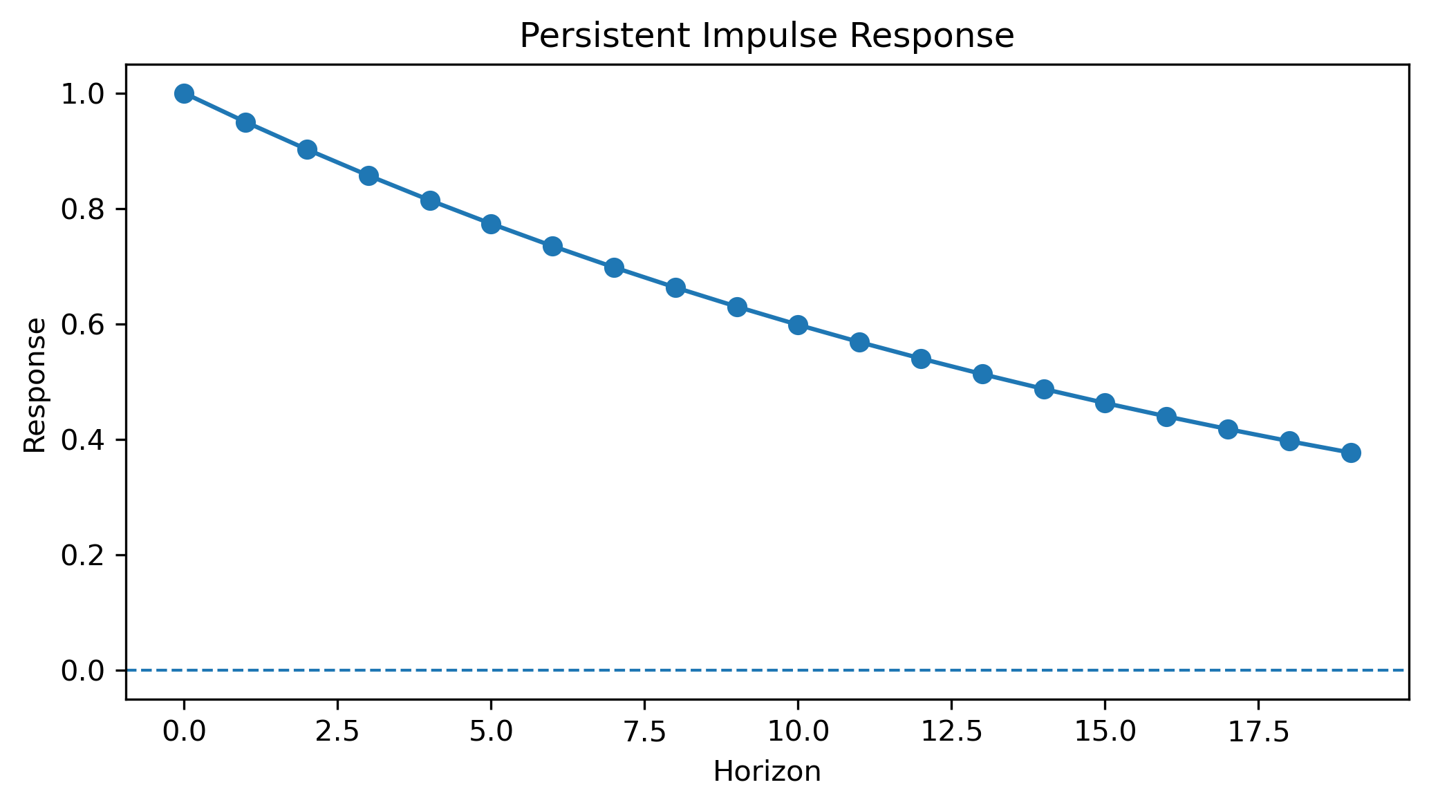

Oscillating Response¶

Some systems overshoot and oscillate before stabilizing.

This may reflect:

delayed adjustment,
cyclical dynamics,
or strong feedback effects.

h = np.arange(20)

irf = np.exp(-0.15*h) * np.cos(1.2*h)

plt.figure(figsize=(7,4))

plt.plot(h, irf, marker="o")

plt.axhline(0, linestyle="--", linewidth=1)

plt.title("Oscillating Impulse Response")
plt.xlabel("Horizon")
plt.ylabel("Response")

plt.tight_layout()

plt.savefig("figs/ch23/oscillating_irf.png",
            dpi=300,
            bbox_inches="tight")

plt.close()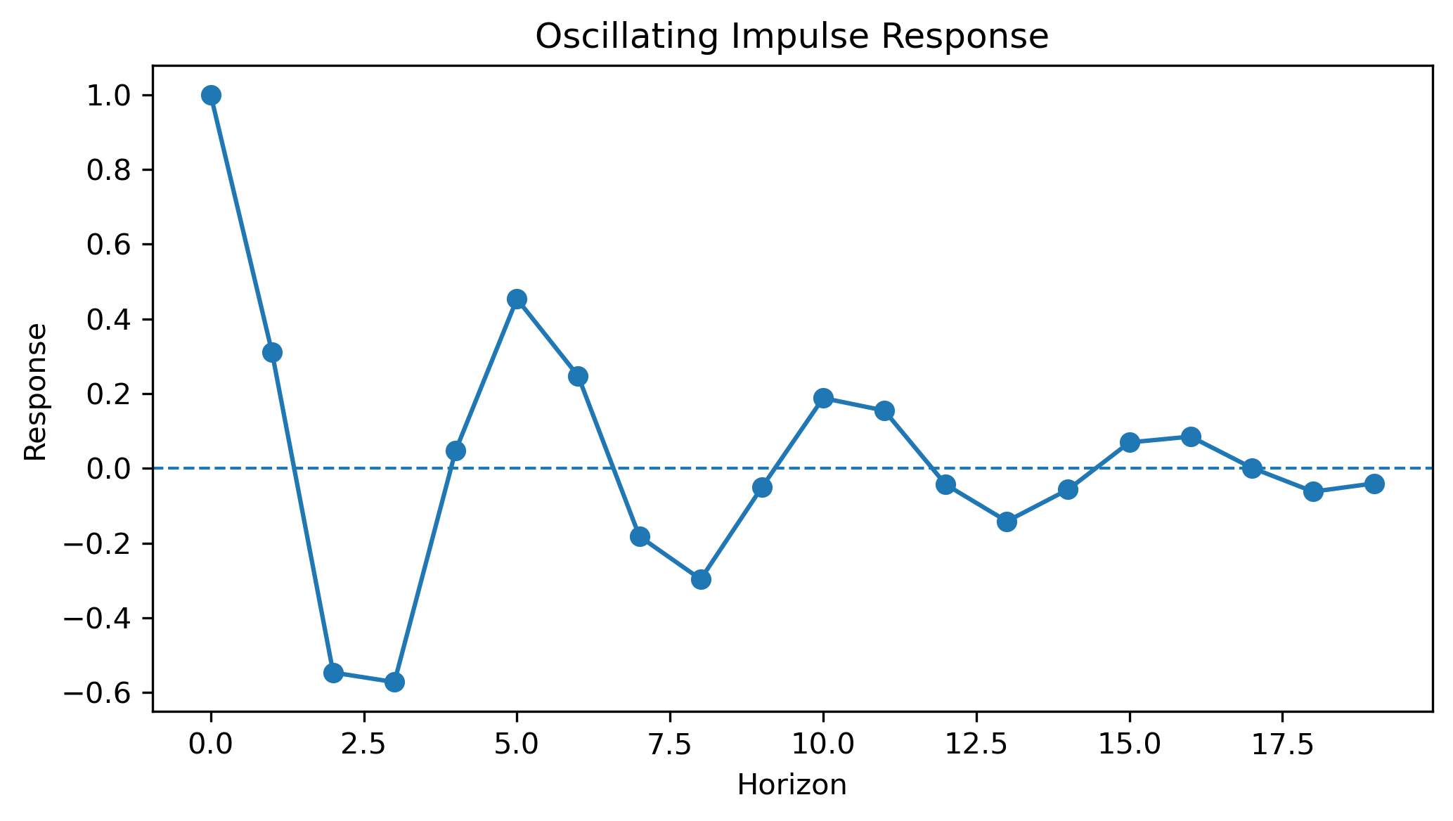

Explosive Response¶

An unstable system may produce impulse responses that grow through time.

This suggests:

instability,
explosive dynamics,
or misspecification.

h = np.arange(12)

irf = 1.15**h

plt.figure(figsize=(7,4))

plt.plot(h, irf, marker="o")

plt.axhline(0, linestyle="--", linewidth=1)

plt.title("Explosive Impulse Response")
plt.xlabel("Horizon")
plt.ylabel("Response")

plt.tight_layout()

plt.savefig("figs/ch23/explosive_irf.png",
            dpi=300,
            bbox_inches="tight")

plt.close()

23.8 Why Orthogonalization Is Necessary¶

A major complication arises because VAR shocks are often correlated.

For example:

stock-market shocks,
volatility shocks,
and interest-rate shocks

may occur simultaneously.

This creates an important problem.

This is the motivation for orthogonalization.

23.9 Cholesky Decomposition¶

One common solution is:

Cholesky decomposition

This transforms correlated shocks into orthogonal shocks.

Intuition¶

Suppose stock returns and volatility both move unexpectedly today.

Cholesky decomposition attempts to separate:

the pure return shock,
from the pure volatility shock.

This allows impulse responses to trace cleaner dynamic effects.

23.10 Ordering and Identification¶

Orthogonalized impulse responses depend on variable ordering.

Example ordering:

returns
volatility
interest rate

This ordering implicitly imposes assumptions about contemporaneous relationships.

For example:

returns may affect volatility immediately,
but volatility may affect returns only with delay.

Why Ordering Matters¶

Different orderings may produce:

different impulse responses,
different persistence patterns,
and different economic conclusions.

This is one reason IRFs should be interpreted carefully.

23.11 Structural Interpretation¶

Reduced-form VARs describe:

dynamic dependence,
correlations,
and propagation patterns.

But economists are often interested in structural interpretation.

For example:

What is a monetary policy shock?

Answering this requires economic theory and identifying assumptions.

Structural interpretation requires assumptions about the economic system.

Structural interpretation requires assumptions.

23.12 Confidence Intervals and Uncertainty¶

Impulse responses are estimated statistically.

Therefore they contain uncertainty.

Confidence intervals help assess statistical precision.

Interpretation¶

Wide confidence bands imply:

substantial uncertainty,
lower precision,
and weaker statistical confidence.

Responses close to zero may not be economically meaningful.

23.13 Estimating IRFs in Python¶

We now estimate impulse responses using a financial VAR system.

The system contains:

SPY daily log returns,
and a rolling volatility proxy.

This example is useful because:

financial shocks often propagate dynamically,
volatility is highly persistent,
and responses are visually intuitive.

import yfinance as yf
import pandas as pd
import numpy as np
import matplotlib.pyplot as plt

from statsmodels.tsa.api import VAR

# Download data
spy = yf.download(
    "SPY",
    start="2015-01-01",
    auto_adjust=False
)

# Compute returns
returns = 100 * np.log(
    spy["Adj Close"] /
    spy["Adj Close"].shift(1)
)

returns = returns.dropna()

# Volatility proxy
volatility = returns.rolling(20).std()

# Combine variables
data = pd.concat(
    [returns, volatility],
    axis=1
)

data.columns = [
    "Returns",
    "Volatility"
]

data = data.dropna()

# Estimate VAR
model = VAR(data)

results = model.fit(2)

# Impulse responses
irf = results.irf(12)

fig, axes = plt.subplots(
    2,2,
    figsize=(10,8),
    facecolor="white"
    )

# plt.style.use("default")
irf.plot()

plt.savefig("figs/ch23/irf.png", dpi=300, bbox_inches="tight")
plt.close()   # replace with plt.show()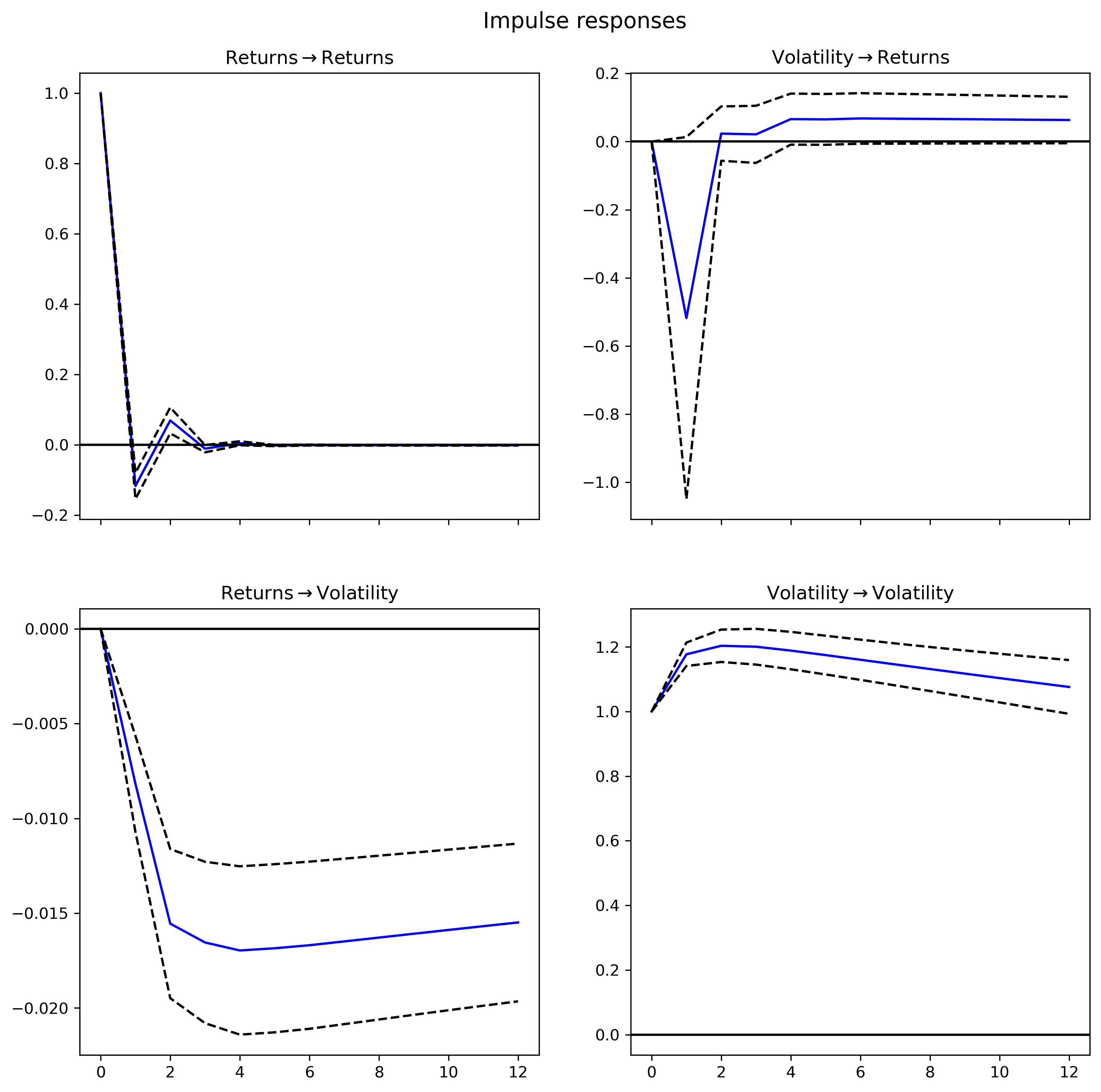

23.14 Interpreting the IRF Results¶

Figure above shows impulse responses for the VAR system containing:

stock returns,
and volatility.

Several important dynamic patterns emerge.

Returns Shock → Returns¶

The response of returns to their own shock decays very quickly.

This suggests:

weak persistence in returns,
rapid adjustment,
and relatively short-lived shocks.

Volatility Shock → Volatility¶

Volatility responses are much more persistent.

The effects decay only gradually through time.

This is one reason volatility modeling becomes especially important in finance.

Cross-Variable Responses¶

The off-diagonal impulse responses show how shocks propagate across variables.

For example:

return shocks influence future volatility,
volatility shocks influence future returns.

This illustrates the dynamic feedback captured by VAR systems.

Confidence Bands¶

The dashed lines represent confidence intervals.

Wide confidence bands imply:

greater uncertainty,
and less statistical precision.

Responses close to zero may not be economically meaningful.

General Interpretation¶

Impulse responses help answer questions such as:

How large are shock effects?
How long do effects persist?
Do shocks disappear quickly or slowly?
Are responses economically plausible?

23.15 Forecast Error Variance Decomposition (FEVD)¶

Impulse responses show how shocks propagate dynamically.

Another important question is:

Forecast Error Variance Decomposition (FEVD) helps answer this question.

FEVD measures how much forecast uncertainty comes from different shocks.

Intuition¶

Suppose volatility forecasts are highly uncertain.

FEVD asks:

how much uncertainty comes from volatility shocks?
how much comes from return shocks?
which shocks dominate over time?

23.16 Interpreting FEVD Results¶

Impulse responses are especially useful because they connect:

data,
dynamics,
and economic theory.

Examples include:

monetary transmission,
fiscal policy effects,
exchange-rate dynamics,
financial contagion.

FEVD tables summarize the relative importance of different shocks.

For example:

volatility shocks may dominate short-run volatility forecasts,
while return shocks may become more important over longer horizons.

23.17 Impulse Responses and Economic Theory¶

Suppose central banks unexpectedly raise interest rates.

Possible impulse responses:

Variable	Possible Response
inflation	declines gradually
GDP	slows
unemployment	rises
exchange rate	appreciates

Delayed Effects¶

Many macroeconomic responses occur only after several periods.

This is sometimes called:

policy transmission lag

23.18 Impulse Responses in Finance¶

IRFs are also widely used in finance.

Examples include:

volatility spillovers,
stock market contagion,
oil-price shocks,
exchange-rate transmission.

Example¶

Question:

How does a U.S. market shock affect Asian stock markets?

VAR and IRF methods are commonly used to study such problems.

23.19 IRFs and Stability¶

In stable systems:

impulse responses eventually converge toward zero.

In unstable systems:

responses may explode.

23.20 Generalized Impulse Responses¶

Standard orthogonalized IRFs depend on ordering assumptions.

An alternative approach is Generalized Impulse Responses

Generalized IRFs reduce sensitivity to variable ordering.

Trade-Off¶

Orthogonalized IRFs:

are easier to interpret structurally,
but depend heavily on ordering.

Generalized IRFs:

reduce ordering sensitivity,
but may be harder to interpret economically.
Different identification approaches may produce different impulse responses.

23.21 Gretl Example: Impulse Responses¶

Gretl provides built-in tools for IRF analysis.

Step 1¶

Estimate a VAR model.

Menu:

Model → Time Series → VAR

Step 2¶

From the VAR output window:

Analysis → Impulse responses

Step 3¶

Choose:

shock variable,
response variable,
forecast horizon,
confidence intervals.

[GRETL Screenshot Placeholder: IRF settings]

23.22 Reading IRF Graphs¶

Typical IRF graphs show:

horizontal axis = time horizon,
vertical axis = response magnitude.

The zero line is especially important.

23.23 Common Mistakes¶

23.24 Looking Ahead¶

Impulse responses allow us to move from:

toward:

The next chapter introduces Vector Error Correction Models (VECMs), which combine:

short-run dynamics,
long-run equilibrium,
and multivariate adjustment mechanisms

within a unified framework.

We will move from

temporary dynamic interactions

toward:

long-run equilibrium systems.

Key Takeaways¶

Concept Check¶

Basic¶

What is an impulse response function (IRF)?
What does a “shock” represent in a VAR model?
Why are IRFs used instead of directly interpreting VAR coefficients?

Intuition¶

Explain the “stone in water” analogy for impulse responses.
Why do economic shocks often have effects over multiple periods?
What does it mean for a shock to “propagate” through a system?

Dynamics¶

What is the difference between:
- contemporaneous effects
- lagged effects
Why do impulse responses often decay over time?

Challenge¶

What does it mean if an impulse response does not decay?

Interpretation & Practice¶

An IRF shows:

a positive initial response
gradual decay to zero
- What does this imply?

An IRF shows a negative response after a positive shock.
- What does this suggest about the relationship?
An IRF oscillates before stabilizing.
- What might this indicate?
An IRF is close to zero at all horizons.
- What does this imply?

Persistence¶

A shock has effects that persist for many periods.
- What does this suggest about the system?
A shock disappears quickly.
- What does this imply?

Confidence Bands¶

Confidence intervals are wide.
- What does this imply?
Confidence bands include zero.
- What does this suggest?

Challenge¶

Why should IRFs always be interpreted together with confidence intervals?

Orthogonalization & Identification¶

Why are VAR shocks often correlated?
What is orthogonalization?
What does Cholesky decomposition do?

Ordering¶

Why does variable ordering matter?
What assumption is made when a variable is ordered first?
What assumption is made when a variable is ordered last?

Interpretation¶

Why are IRFs not automatically causal?

Challenge¶

How can different ordering assumptions change conclusions?

Numerical & Graph Interpretation¶

Interpreting an Impulse Response Function¶

Consider the following impulse response function:

import numpy as np
import matplotlib.pyplot as plt

horizon = np.arange(10)

# stylized IRF: rise → peak → decay
irf = [0.0, 0.5, 0.9, 1.2, 1.0, 0.7, 0.4, 0.2, 0.1, 0.0]

plt.figure(figsize=(8,4))
plt.plot(horizon, irf, marker='o')

plt.axhline(0, linestyle='--', linewidth=1)

plt.title("Stylized Impulse Response Function")
plt.xlabel("Horizon")
plt.ylabel("Response")

plt.tight_layout()

plt.savefig("figs/ch23/irf_Q.png", dpi=300, bbox_inches="tight")
plt.close()   # replace with plt.show()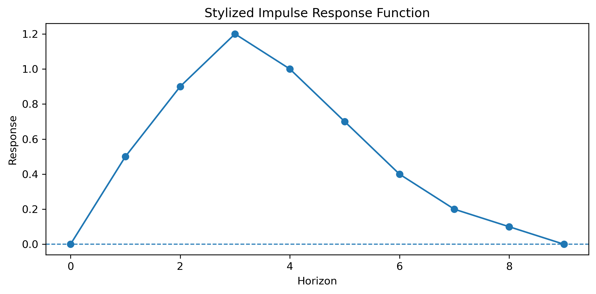

Describe the pattern of the impulse response.
At what period does the response peak?
Does the effect persist or disappear quickly?
What does this suggest about the dynamic impact of the shock?

Reading an IRF¶

Suppose an IRF shows:

initial increase
peak after 3 periods
slow decline

What does this suggest?

Cumulative Effects¶

Why might we use cumulative impulse responses?
Suppose cumulative IRF increases steadily.

What does this imply?

Stability¶

Suppose IRFs grow larger over time.

What does this imply?

Comparison¶

Two IRFs:

one decays quickly
one decays slowly

Which system is more persistent?

Challenge¶

Suppose a shock produces different responses depending on ordering.

What does this suggest?

Appendix 23A — Orthogonalized vs Generalized IRFs¶

Orthogonalized IRFs:

rely on Cholesky decomposition,
depend on variable ordering.

Generalized IRFs:

reduce ordering sensitivity,
but may be harder to interpret structurally.

Different approaches may produce somewhat different results.

Appendix 23B — Why Impulse Responses Became Popular¶

VAR coefficient matrices are often difficult to interpret directly.

Impulse responses became popular because they:

summarize complex dynamics visually,
describe propagation mechanisms,
connect statistical models with economic narratives.

They transformed VAR analysis from:

large coefficient tables

into dynamic economic interpretation.