Chapter 24 — Vector Error Correction Models (VECM)

In earlier chapters, we studied:

nonstationary time series,
cointegration,
and error correction models (ECMs).

We saw that some variables may drift over time individually, yet still maintain stable long-run relationships.

Examples include:

money supply and prices,
GDP and credit,
exchange rates and inflation,
stock indices across markets.

In the previous two chapters, we introduced VAR models for multivariate dynamics.

But standard VAR models become problematic when variables are:

This chapter introduces the solution:

The answer is the:

VECMs combine:

cointegration,
VAR dynamics,
and equilibrium adjustment

within a unified framework.

Throughout the chapter, we use Thai macroeconomic data as a running example.

Learning Objectives¶

By the end of this chapter, you should be able to:

explain the intuition behind VECMs
distinguish VARs from VECMs
understand equilibrium correction
interpret error correction terms
estimate VECMs
understand cointegration rank
interpret adjustment coefficients
perform Johansen cointegration tests
analyze long-run and short-run dynamics jointly

24.1 Why VAR Models Are Not Enough¶

Recall that standard VAR models usually require stationary variables.

But many macroeconomic variables are:

trending,
persistent,
integrated of order one.

Examples include:

CPI,
money supply,
nominal GDP,
price levels.

The Problem¶

If we estimate a VAR using nonstationary variables:

spurious relationships may emerge,
standard inference becomes unreliable.

One solution is:

But differencing creates another problem.

For example:

inflation and money supply may move together over decades,
GDP and credit may share long-run trends.

Pure differencing may destroy this information.

24.2 Cointegration Revisited¶

Suppose two variables:

trend upward individually,
but maintain stable long-run relationships.

Then they may be:

Thai Macro Example¶

Suppose:

Thai CPI,
and broad money supply (BM)

both trend upward through time.

Even though both series are nonstationary individually, they may still move together in the long run because:

monetary expansion influences prices,
inflation affects money demand,
central bank policy links the two variables.

24.3 From ECM to VECM¶

Recall the simple ECM:

\Delta y_t = \alpha + \beta \Delta x_t + \lambda (y_{t-1}-\gamma x_{t-1}) + u_t

The term:

(y_{t-1}-\gamma x_{t-1})

measures deviation from long-run equilibrium.

Extending to Multiple Variables¶

A VECM generalizes this idea to:

several variables,
several equations,
multiple equilibrium relationships.

24.4 Intuition of the VECM¶

A VECM combines:

short-run dynamics,
and long-run equilibrium adjustment.

24.5 Rubber-Band Analogy¶

A useful analogy is:

Short-run shocks may pull variables apart.

But the rubber band creates pressure toward long-run equilibrium.

This is precisely the role of the:

24.6 Thai Macro Example¶

We now examine Thai macroeconomic variables.

Our dataset contains:

CPI,
broad money supply (BM),
real GDP,
GDP deflator.

Loading the Data¶

import pandas as pd
from io import StringIO

data_text = """
year,cpi,BM_,gdp_r
1991,50.70,204654.4084,38.23977231
1992,52.80,237852.2993,41.58407966
1993,54.50,272926.6351,43.40940123
1994,57.30,302096.2673,46.88149708
1995,60.60,355694.6742,50.68815184
1996,64.10,393470.4887,53.55329227
1997,67.70,470396.7099,52.07872106
1998,73.10,517768.2452,48.10357948
1999,73.30,537431.8537,50.30235946
2000,74.50,563808.6622,52.54366163
2001,75.70,594569.9039,54.3535078
2002,76.20,617075.0830,57.69600000
2003,77.60,707867.6497,61.84370042
2004,79.80,747291.5105,65.73352411
2005,83.40,792795.6350,68.48596905
2006,87.30,857454.6312,71.88876509
2007,89.20,911063.5572,75.79552154
2008,94.10,994546.5100,77.10330582
2009,93.30,1061828.8660,76.53419316
2010,96.33,1178006.9540,82.27951477
2011,100.00,1356089.1230,82.96559013
2012,103.02,1496760.9480,88.96449269
2013,105.27,1606334.2890,91.36862416
2014,107.26,1681035.3120,92.11543151
"""

thai = pd.read_csv(
    StringIO(data_text)
)

thai.head()

Plotting CPI and Broad Money¶

Because CPI and broad money are measured on very different scales, it is useful to display them using two vertical axes.

import matplotlib.pyplot as plt

fig, ax1 = plt.subplots(figsize=(10,5))

# ==========================================
# Left Axis: CPI
# ==========================================

ax1.plot(
    thai["year"],
    thai["cpi"],
    linewidth=2,
    label="CPI"
)

ax1.set_xlabel("Year")

ax1.set_ylabel("CPI")

# ==========================================
# Right Axis: Broad Money
# ==========================================

ax2 = ax1.twinx()

ax2.plot(
    thai["year"],
    thai["BM_"],
    linewidth=2,
    linestyle="--",
    label="Broad Money"
)

ax2.set_ylabel("Broad Money")

# ==========================================
# Title
# ==========================================

plt.title("Thailand: CPI and Broad Money")

# ==========================================
# Combined Legend
# ==========================================

lines1, labels1 = ax1.get_legend_handles_labels()

lines2, labels2 = ax2.get_legend_handles_labels()

ax1.legend(
    lines1 + lines2,
    labels1 + labels2,
    loc="upper left"
)

plt.savefig("figs/ch24/cpiBM.png", dpi=300, bbox_inches="tight")
plt.close()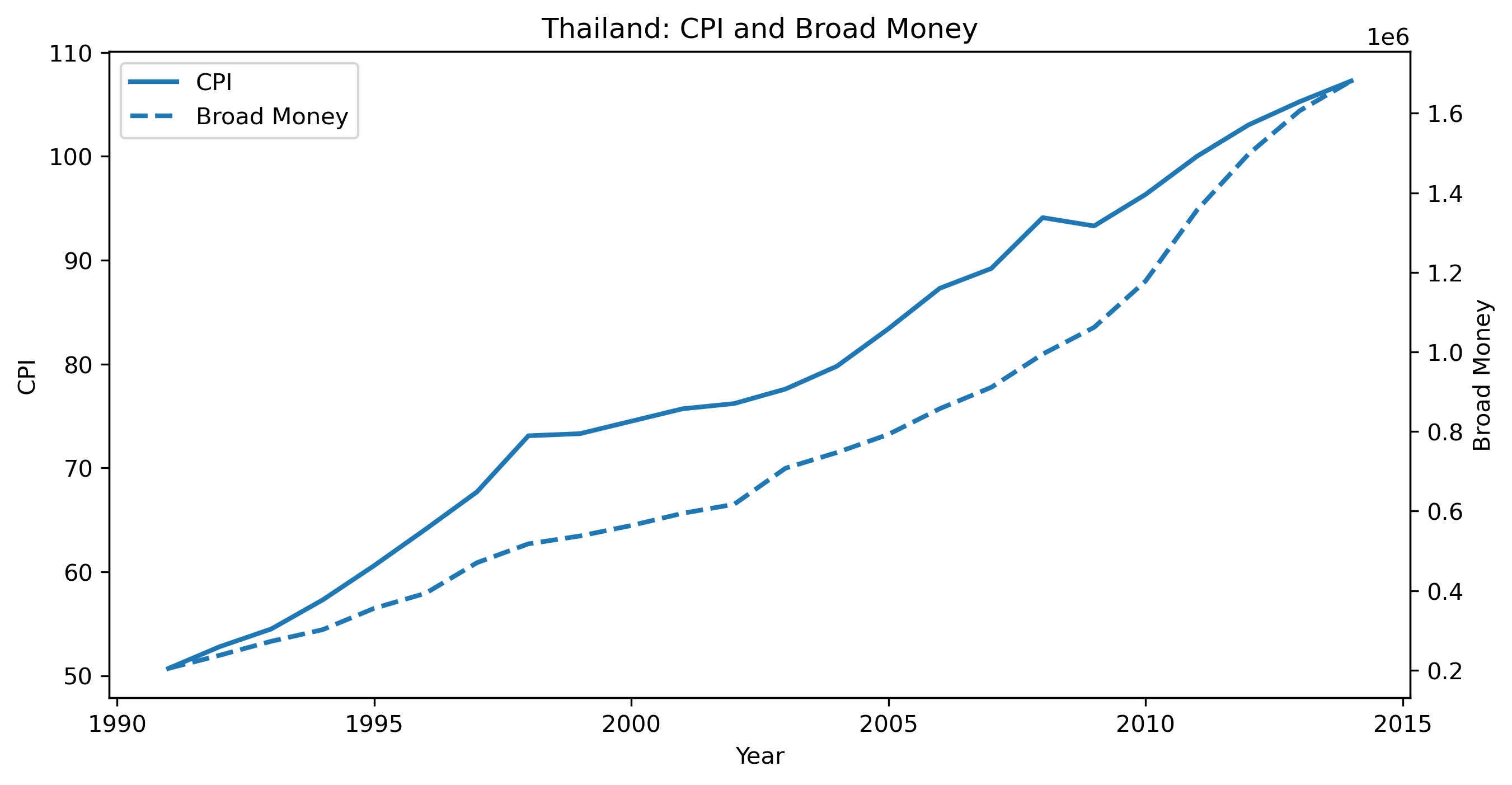   # replace with plt.show()

This immediately raises important questions:

Are the series nonstationary?
Do they share a common long-run equilibrium relationship?

24.7 The VECM Representation¶

A VECM may be written as:

\Delta Y_t = \Pi Y_{t-1} + \Gamma_1 \Delta Y_{t-1} + \cdots + \Gamma_{p-1}\Delta Y_{t-p+1} + u_t

where:

$\Delta Y_t$ = differenced variables,
$\Pi Y_{t-1}$ = equilibrium correction,
$\Gamma_i$ = short-run dynamics.

24.8 The Error Correction Matrix¶

The matrix:

\Pi

contains the long-run information.

It can be decomposed as:

\Pi = \alpha \beta'

where:

$\beta$ = cointegration vectors,
$\alpha$ = adjustment coefficients.

24.9 Cointegration Rank¶

An important concept is:

Interpretation¶

Rank	Interpretation
0	no cointegration
1	one long-run equilibrium relationship
multiple	several equilibrium relationships

24.10 Short-Run vs Long-Run Dynamics¶

VECMs separate:

short-run movements,
and long-run adjustment.

Short Run¶

Captured by:

\Gamma_i \Delta Y_{t-i}

Long Run¶

Captured by:

\Pi Y_{t-1}

24.11 The Johansen Cointegration Test¶

The Johansen procedure is the standard method for testing cointegration in multivariate systems.

24.12 Trace and Maximum Eigenvalue Tests¶

The Johansen method commonly reports:

trace statistics,
maximum eigenvalue statistics.

These are used to test:

24.13 Johansen Test in Python¶

We now test for cointegration between:

Thai CPI,
and broad money supply.

from statsmodels.tsa.vector_ar.vecm import coint_johansen

data = thai[["cpi","BM_"]].dropna()

johansen_test = coint_johansen(
    data,
    det_order=0,
    k_ar_diff=2
)

print(johansen_test.lr1)

[7.30400737e+00 1.97612579e-03]

24.14 Estimating a VECM in Python¶

We now estimate a VECM.

from statsmodels.tsa.vector_ar.vecm import VECM

model = VECM(
    data,
    k_ar_diff=2,
    coint_rank=1
)

results = model.fit()

print(results.summary())

Det. terms outside the coint. relation & lagged endog. parameters for equation cpi
==============================================================================
                 coef    std err          z      P>|z|      [0.025      0.975]
------------------------------------------------------------------------------
L1.cpi        -0.0496      0.233     -0.213      0.831      -0.505       0.406
L1.BM_       1.14e-05   1.23e-05      0.929      0.353   -1.26e-05    3.54e-05
L2.cpi         0.1963      0.246      0.797      0.426      -0.287       0.679
L2.BM_     -6.798e-06   1.28e-05     -0.531      0.596   -3.19e-05    1.83e-05
Det. terms outside the coint. relation & lagged endog. parameters for equation BM_
==============================================================================
                 coef    std err          z      P>|z|      [0.025      0.975]
------------------------------------------------------------------------------
L1.cpi     -6233.3424   4210.754     -1.480      0.139   -1.45e+04    2019.584
L1.BM_         0.6357      0.222      2.863      0.004       0.200       1.071
L2.cpi     -4809.5980   4462.296     -1.078      0.281   -1.36e+04    3936.341
L2.BM_         0.1610      0.232      0.694      0.488      -0.294       0.616
                Loading coefficients (alpha) for equation cpi                 
==============================================================================
                 coef    std err          z      P>|z|      [0.025      0.975]
------------------------------------------------------------------------------
ec1            0.0349      0.017      1.999      0.046       0.001       0.069
                Loading coefficients (alpha) for equation BM_                 
==============================================================================
                 coef    std err          z      P>|z|      [0.025      0.975]
------------------------------------------------------------------------------
ec1          852.4602    316.000      2.698      0.007     233.112    1471.808
          Cointegration relations for loading-coefficients-column 1           
==============================================================================
                 coef    std err          z      P>|z|      [0.025      0.975]
------------------------------------------------------------------------------
beta.1         1.0000          0          0      0.000       1.000       1.000
beta.2     -3.752e-05   3.11e-05     -1.207      0.228   -9.85e-05    2.34e-05
==============================================================================

24.15 Error Correction Terms¶

A crucial component is the:

This measures deviation from long-run equilibrium.

Example¶

Suppose money supply rises much faster than prices.

The VECM captures pressure for future adjustment.

Possible responses include:

inflation increasing,
money growth slowing,
or both.

24.16 Adjustment Speeds¶

Adjustment coefficients measure:

Large Adjustment Coefficient¶

fast correction,
rapid equilibrium restoration.

Small Adjustment Coefficient¶

slow adjustment,
persistent disequilibrium.

24.17 Impulse Responses in VECMs¶

Impulse responses can also be generated from VECMs.

However, the responses now reflect:

short-run dynamics,
and long-run equilibrium structure.

24.18 Forecasting with VECMs¶

VECMs are often superior to differenced VARs when cointegration exists.

Why?

Because they preserve:

equilibrium relationships,
long-run information,
adjustment dynamics.

24.19 Financial Applications of VECMs¶

VECMs are widely used in finance.

Examples include:

pairs trading,
stock market integration,
exchange-rate systems,
interest-rate term structure.

Example: Pairs Trading¶

If two stock prices are cointegrated:

temporary deviations may create trading opportunities.

This idea underlies many statistical arbitrage strategies.

24.20 Macroeconomic Applications¶

VECMs are also widely used in macroeconomics.

Examples include:

money demand,
purchasing power parity,
inflation dynamics,
monetary policy transmission.

24.21 VECM vs VAR¶

Feature	VAR	VECM
stationary variables	✓	✓
nonstationary variables	problematic	✓
cointegration	ignored	incorporated
long-run equilibrium	no	yes

24.22 Gretl Example: Johansen Test¶

Gretl provides built-in cointegration tools.

Step 1¶

Load multiple nonstationary variables.

Step 2¶

Menu:

Model → Time Series → VECM

Step 3¶

Select:

lag length,
deterministic terms,
cointegration rank.

[GRETL Screenshot Placeholder: Johansen test output]

Gretl Example: Estimating a VECM¶

After selecting rank and lags:

GRETL estimates:

cointegration vectors,
adjustment coefficients,
short-run dynamics.

[GRETL Screenshot Placeholder: VECM estimation output]

24.23 Common Mistakes¶

24.25 Looking Ahead¶

This concludes our introduction to multivariate time series models.

We have now studied:

VAR models,
impulse responses,
and VECMs.

The next part of the book turns toward:

volatility,
ARCH models,
and GARCH models.

We shift from modeling:

toward modeling:

of financial time series.

Key Takeaways¶

Concept Check¶

Basic¶

What is a Vector Error Correction Model (VECM)?
How does a VECM differ from a standard VAR model?
When should a VECM be used instead of a VAR?

Intuition¶

Why is differencing alone not sufficient when variables are cointegrated?
What is the economic meaning of cointegration in a multivariate system?
Explain the “rubber band” analogy in the context of VECM.

Structure¶

What are the two main components of a VECM?
What does the term $\Pi Y_{t-1}$ represent?
What do the $\Gamma_i$ terms capture?

α and β¶

What does the matrix $\beta$ represent?
What does the matrix $\alpha$ represent?
Why is the decomposition $\Pi = \alpha \beta'$ important?

Challenge¶

Why is it not enough to estimate a VAR in differences when variables are cointegrated?

Interpretation & Practice¶

A system shows strong cointegration.

What does this imply about long-run relationships?

The cointegration rank is zero.

What does this imply?

The cointegration rank is one.

What does this imply?

Adjustment coefficients are large in magnitude.

What does this suggest?

Adjustment coefficients are close to zero.

What does this imply?

Error Correction¶

The error correction term is significant in one equation but not the other.

What does this imply?

A variable does not respond to disequilibrium.

What might this suggest?

Economic Interpretation¶

CPI and money supply are cointegrated.

What does this imply about long-run behavior?

You estimate a system with:

CPI
money supply
GDP

You find:

cointegration rank = 1
CPI adjusts strongly
money supply adjusts weakly

What does this suggest about economic dynamics?
Which variable leads the system?
Which variable follows?

Challenge¶

Why is VECM considered a “restricted VAR”?

Numerical Practice¶

Cointegration Logic¶

Suppose:

$x_t \sim I(1)$
$y_t \sim I(1)$
one cointegrating vector exists

What does this imply?

Rank Interpretation¶

Suppose a system of 3 variables has:

cointegration rank = 2

How many long-run relationships exist?

Adjustment Coefficients¶

Suppose:

\alpha = \begin{pmatrix} -0.3 \\ 0.0 \end{pmatrix}

Which variable adjusts to equilibrium?
Which does not?

Interpretation¶

Suppose:

\beta' Y_{t-1} = y_{t-1} - 2x_{t-1}

What does this represent?

Short vs Long Run¶

Why is it important to include both:

$\Delta Y_t$ terms
and $\Pi Y_{t-1}$ terms?

Diagnostics¶

Suppose cointegration is ignored and a VAR in differences is estimated.

What information is lost?

Challenge¶

Suppose cointegration rank is incorrectly specified.

What problems might arise?

Johansen Test Interpretation¶

What does the Johansen test estimate?
What is the difference between:

trace test
maximum eigenvalue test

Interpretation¶

Suppose the test suggests rank = 1.

What does this imply?

Suppose test statistics are small.

What does this suggest?

Challenge¶

Why is determining the correct cointegration rank important?

IRF & Forecasting in VECM¶

How do impulse responses differ in VECM vs VAR?
Why do long-run relationships affect IRFs?

Interpretation¶

A shock causes variables to deviate, then gradually return.

What does this reflect?

Why might VECM forecasts outperform differenced VAR forecasts?

Challenge¶

Why is long-run information valuable in forecasting?

Appendix 24A — Relationship Between VAR and VECM¶

A VECM can be derived algebraically from a VAR expressed in levels.

Suppose:

Y_t = A_1 Y_{t-1} + \cdots + A_p Y_{t-p} + u_t

Rewriting the system in differences produces:

short-run difference terms,
and a long-run equilibrium term.

This decomposition leads directly to the VECM representation.

Appendix 24B — Why Cointegration Matters Economically¶

Cointegration matters because many economic variables are tied together by long-run equilibrium forces.

Examples include:

money and prices,
income and consumption,
exchange rates and inflation.

Without equilibrium adjustment:

economic systems could drift apart indefinitely.

Cointegration formalizes the idea that: