Chapter 2 — Returns and Financial Data
Financial markets generate enormous amounts of time series data.
Every trading day produces new observations on:
stock prices
exchange rates
bond yields
commodity prices
cryptocurrency prices
market indices
But financial analysts rarely work directly with prices alone.
Instead, they usually focus on returns.
This chapter introduces the basic structure of financial data and the logic of financial returns.
We study:
simple returns
log returns
compounding
adjusted prices
short selling
stylized facts of financial returns
We also begin working directly with real financial data using Python and Yahoo Finance.
Learning Objectives
By the end of this chapter, you should be able to:
distinguish prices from returns
compute simple and log returns
explain compounding intuitively
explain why log returns are useful
understand adjusted prices
explain the logic of short selling
identify stylized facts of financial returns
download and visualize financial data using Python
2.1 Financial Prices
A financial price represents the market value of an asset at a particular moment in time.
Examples include:
stock prices
exchange rates
gold prices
bond prices
cryptocurrency prices
We often denote the price at time as:
For example:
| Day | Price |
|---|---|
| Monday | 100 |
| Tuesday | 103 |
| Wednesday | 101 |
Why Prices Alone Are Not Enough
Suppose:
Stock A rises from 10 to 11
Stock B rises from 100 to 101
Both increased by 1 unit.
But the economic significance is very different.
This motivates the concept of returns.
2.2 Simple Returns
For a price series , the simple return is:
Simple returns measure proportional price change.
Example
Suppose:
Then:
or:
2.3 Positive and Negative Returns
Returns may be positive or negative.
| Price Movement | Return |
|---|---|
| price rises | positive return |
| price falls | negative return |
Example:
Then:
or:
2.4 Gross Returns
Sometimes it is useful to work with the gross return:
Examples:
| Simple Return | Gross Return |
|---|---|
| 5% | 1.05 |
| -3% | 0.97 |
Gross returns are especially useful for compounding.
2.5 Compounding Intuition
Suppose an investment earns:
10% in year 1
10% in year 2
Starting from:
After year 1:
After year 2:
Overall growth is therefore:
or:
2.6 Why You Cannot Simply Average Returns
Consider the following price series:
| Year | Price |
|---|---|
| 2020 | 100 |
| 2021 | 80 |
| 2022 | 100 |
The price:
falls from 100 to 80
then rises from 80 back to 100
The simple returns are:
| Period | Return |
|---|---|
| 2021 | -20% |
| 2022 | +25% |
Now notice something interesting:
But the investment did not earn 5%.
The final price returned exactly to the starting value.
Total return is therefore:
This is one of the main motivations for log returns.
2.7 Log Returns
Financial analysts often work with log returns instead of simple returns.
The log return is:
Equivalently:
where:
denotes the simple return.
Example
Suppose:
Then:
or approximately:
2.8 Why Log Returns Matter
At first glance, log returns may seem unnecessarily complicated.
Why not simply use percentage returns?
The answer lies in compounding.
Suppose returns over multiple periods are:
The compounded gross return is:
Taking logs:
Using logarithm rules:
This property is called:
time additivityand is one of the main reasons log returns are widely used in finance and econometrics.
2.9 Simple Returns vs Log Returns
| Feature | Simple Returns | Log Returns |
|---|---|---|
| intuitive | ✓ | |
| additive through time | ✓ | |
| commonly used in finance | ✓ | ✓ |
| natural for continuous compounding | ✓ |
2.10 Small-Return Approximation
For small returns:
This approximation is usually very accurate for daily financial returns.
Example
| Simple Return | Log Return |
|---|---|
| 1% | 0.995% |
| 5% | 4.88% |
| 10% | 9.53% |
As returns become larger, the difference becomes more important.
2.11 Long Positions and Short Selling
Most investors profit when prices rise.
This is called a long position.
Long Position
Buy first, sell later.
Profit if price rises.
Short Selling
Short selling reverses the logic.
The investor:
borrows an asset,
sells it,
later buys it back.
Profit occurs if the price falls.
Example
Suppose:
you short sell at 100
later repurchase at 90
Profit:
Risk of Short Selling
Losses from a long position are limited because prices cannot fall below zero.
But short-selling losses can theoretically be unlimited if prices rise dramatically.
2.12 Downloading Financial Data with Python
We now download real financial data using Python.
import yfinance as yf
import matplotlib.pyplot as plt

aapl = yf.download("AAPL", start="2020-01-01", auto_adjust=False)

print(aapl.head())
We use
auto_adjust=Falseto get the Adjusted Closing price.
Understanding the Columns
Yahoo Finance typically provides:
| Variable | Meaning |
|---|---|
| Open | opening price |
| High | highest price |
| Low | lowest price |
| Close | closing price |
| Adj Close | adjusted closing price |
| Volume | trading volume |
2.13 Adjusted Prices
One of the most important concepts in financial data is the adjusted price.
Stock prices may change because of:
dividends
stock splits
corporate actions
Raw prices therefore may not accurately reflect investor returns.
Example: A 2-for-1 Stock Split
Suppose a company’s stock price evolves as follows:
| Date | Close Price | Shares Held | Investor Wealth |
|---|---|---|---|
| Day 1 | 100 | 1000 | 100,000 |
| Day 2 | 102 | 1000 | 102,000 |
| Day 3 | 105 | 1000 | 105,000 |
Now suppose the company announces a:
2-for-1 stock splitEach shareholder receives:
twice as many shares,
but each share is worth half as much.
After the split:
| Date | Close Price | Shares Held | Investor Wealth |
|---|---|---|---|
| Day 4 | 52.5 | 2000 | 105,000 |
Notice:
Investor wealth is unchanged.
Why Raw Prices Become Misleading
If we looked only at raw prices, we might incorrectly conclude that the stock experienced a:
price crash:
But this is economically incorrect.
The investor is neither richer nor poorer after the split.
Adjusted Prices
Adjusted prices correct for stock splits and other corporate actions.
An adjusted price series might therefore look like:
| Date | Close Price | Trader’s Quantity | Net Worth | Adjusted Close | Daily Return |
|---|---|---|---|---|---|
| Day 1 | 100.0 | 1000 | 100,000 | 50.0 | — |
| Day 2 | 102.0 | 1000 | 102,000 | 51.0 | 2.0% |
| Day 3 | 105.0 | 1000 | 105,000 | 52.5 | 2.9% |
| Day 4 | 52.5 | 2000 | 105,000 | 52.5 | 0.0% |
| Day 5 | 54.0 | 2000 | 108,000 | 54.0 | 2.9% |
Now the artificial price break disappears.
Why Adjusted Prices Matter
Using raw prices incorrectly can produce misleading returns.
Most empirical financial analysis therefore uses:
Adjusted Closerather than raw closing prices.
2.14 Calculating Returns in Python
We now calculate both simple and log returns.
import numpy as np
import pandas as pd

price = [100, 80, 100, 115, 125]
year = [2020, 2021, 2022, 2023, 2024]

df = pd.DataFrame({"price": price}, index=year)

df["simple_return"] = df["price"].pct_change()

df["log_return"] = np.log(
    df["price"] / df["price"].shift(1)
)

df| year | price | simple_return | log_return |
|---|---|---|---|
| 2020 | 100 | NaN | NaN |
| 2021 | 80 | -0.200000 | -0.223144 |
| 2022 | 100 | 0.250000 | 0.223144 |
| 2023 | 115 | 0.150000 | 0.139762 |
| 2024 | 125 | 0.086957 | 0.083382 |
2.15 Cumulative Returns
To compute cumulative growth from simple returns, we compound.
cum_gross = (df["simple_return"] + 1).cumprod()

cum_gross| year | cumulative returns |
|---|---|
| 2020 | NaN |
| 2021 | 0.80 |
| 2022 | 1.00 |
| 2023 | 1.15 |
| 2024 | 1.25 |
Cumulative Log Returns
With log returns, we simply add.
cum_log = df["log_return"].cumsum()

cum_log| year | cumulative log_return |
|---|---|
| 2020 | NaN |
| 2021 | -0.2231436 |
| 2022 | 5.551115e-17 |
| 2023 | 0.1397619 |
| 2024 | 0.2231436 |
Consistency Check
The cumulative log return should equal:
We verify this directly.
np.log(df["price"].iloc[-1]) - np.log(df["price"].iloc[0])np.float64(0.2231435513142097)
Returning to Gross Returns
Exponentiating cumulative log returns recovers total growth.
np.exp(cum_log.iloc[-1])np.float64(1.25)
2.16 Stylized Facts of Financial Returns
Financial returns display several recurring empirical patterns.
These are called stylized facts.
Stylized Fact 1: Returns Are Noisy
Asset returns fluctuate substantially from day to day.
Short-run movements are often difficult to predict.
Stylized Fact 2: Volatility Clustering
Large movements tend to cluster together.
Calm periods are followed by calm periods.
Volatile periods are followed by volatile periods.
This observation motivates ARCH and GARCH models later in the book.
Stylized Fact 3: Fat Tails
Extreme movements occur more often than predicted by the normal distribution.
Examples include:
financial crashes
sudden rallies
market panics
Stylized Fact 4: Asymmetry
Financial markets sometimes fall faster than they rise.
Negative shocks may generate stronger volatility responses than positive shocks.
2.17 Example: Comparing Prices and Returns
import yfinance as yf
import matplotlib.pyplot as plt

aapl = yf.download("AAPL", start="2020-01-01", auto_adjust=False)

prices = aapl["Adj Close", "AAPL"]

returns = prices.pct_change()

fig, ax = plt.subplots(2,1, figsize=(10,7))

ax[0].plot(prices)
ax[0].set_title("Apple Adjusted Prices")

ax[1].plot(returns)
ax[1].set_title("Apple Daily Returns")

plt.tight_layout()

plt.savefig("figs/ch2/aapl.png", dpi=300, bbox_inches="tight")
plt.close()   # replace with plt.show()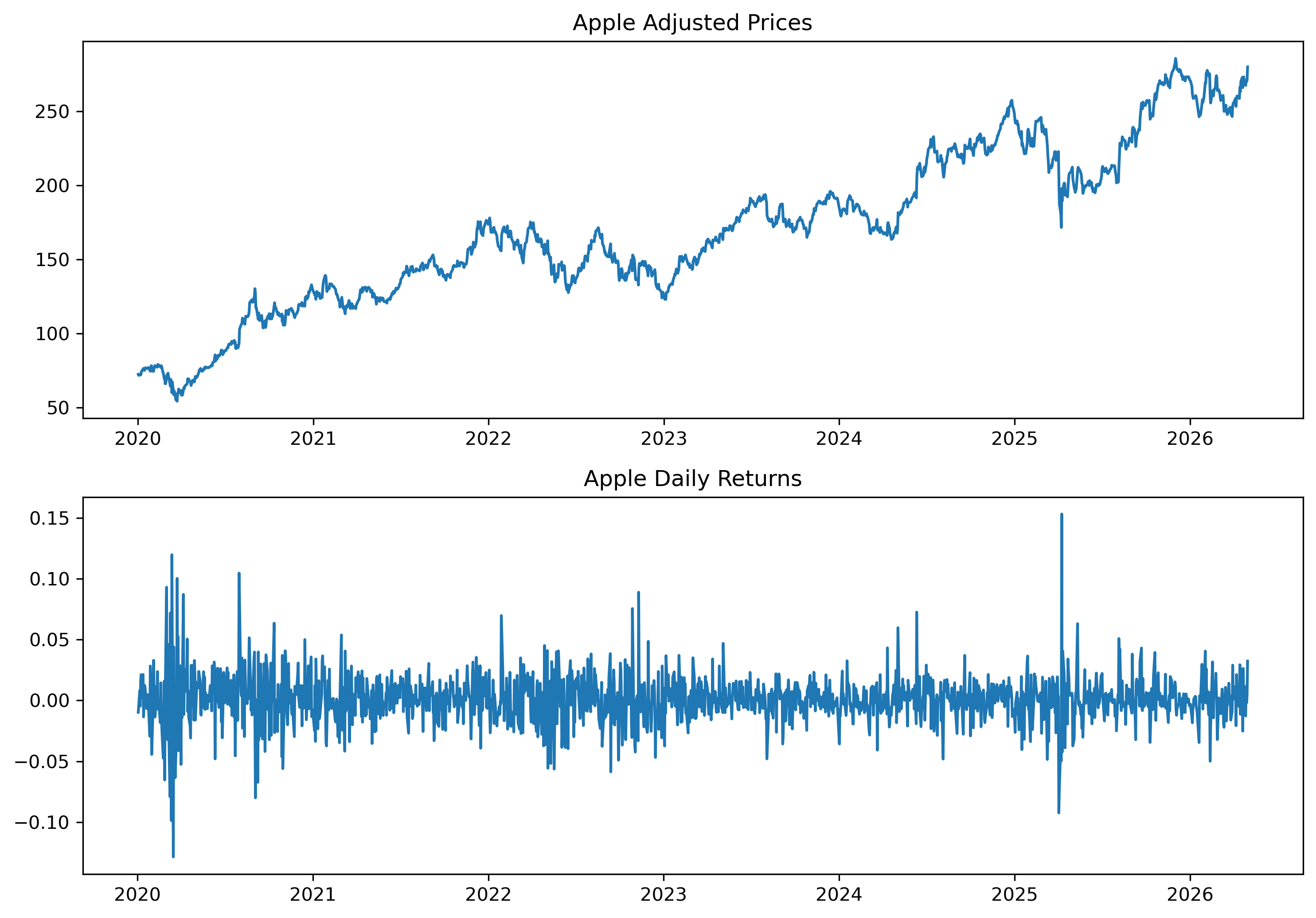
2.18 Gretl Example: Importing Financial Data
Gretl can import financial datasets directly from CSV or Excel files.
Step 1: Download Data
Download data from Yahoo Finance as CSV.
[GRETL Screenshot Placeholder: Yahoo Finance download page]Step 2: Import into GRETL
Menu:
File → Open data → Import
Choose the downloaded CSV file.
[GRETL Screenshot Placeholder: GRETL import window]Step 3: Plot the Series
Select the variable and choose:
Variable → Time series plot
[GRETL Screenshot Placeholder: Financial time series plot]2.19 Common Mistakes
2.20 Looking Ahead
This chapter introduced the foundations of financial time series data.
In the next chapter, we briefly review key ideas from probability and statistics that will be useful throughout the book.
We will study:
randomness
probability distributions
sampling intuition
hypothesis testing
statistical uncertainty
Key Takeaways
Concept Check
Basic
What is the difference between a price and a return?
What is a simple return?
What is a log return?
Intuition
Why are returns often preferred over prices in financial analysis?
What does compounding mean in a financial context?
Why do investors care about percentage changes rather than absolute changes?
Intermediate
How do simple returns and log returns differ in interpretation?
Why are log returns often used in time series modeling?
What is meant by “stylized facts” of financial returns?
Challenge
Suppose a stock price doubles over a year.
What is the simple return?
What is the log return?
Why are they different?
Interpretation & Practice
Consider the following:
Price today = 100
Price tomorrow = 105What is the simple return?
What does this return represent economically?
A stock increases from 100 to 110, then falls back to 100.
What are the simple returns in each period?
What is the total return over the two periods?
What does this illustrate about compounding?
You observe a time series of stock prices that trends upward over time.
What happens to returns when you transform prices into returns?
Why might this be useful?
A histogram of returns shows:
many small values,
a few very large positive and negative values.
What feature of financial data does this illustrate?
Why is this important for modeling?
A time series plot of returns shows periods of calm followed by periods of large fluctuations.
What is this phenomenon called?
Why is it important for risk measurement?
Challenge
Suppose two assets have the same average return, but one has much higher volatility.
Which asset is riskier?
Why might an investor still prefer the lower-volatility asset?
Numerical Practice
Basic
Suppose a stock price moves from 100 to 105.
Compute the simple return.
Express your answer as a percentage.
Suppose a stock price moves from 50 to 55.
Compute the simple return.
Is this higher or lower than in Question 1?
Intermediate
A stock price evolves as follows:
Day Price 0 100 1 110 2 121 Compute the simple return from Day 0 → Day 1.
Compute the simple return from Day 1 → Day 2.
What do you notice?
Using the same data:
Compute the cumulative return from Day 0 → Day 2.
Verify that it matches compounding.
Log Returns
Suppose a stock price moves from 100 to 110.
Compute the log return:
Is it larger or smaller than the simple return?
A stock moves:
100 → 110 → 100
Compute the two simple returns.
Compute the total compounded return.
What do you observe?
Challenge
Suppose returns are:
Day 1: +10%
Day 2: −10%
Compute the final price (starting from 100).
Why is the final value not equal to the initial value?
Suppose daily log returns are:
0.05
0.02
−0.01
Compute the total log return.
What is the advantage of using log returns here?
Appendix 2A — A More Technical Look at Log Returns
This appendix provides a slightly more formal explanation of why log returns are so important in finance and econometrics.
A.1 Continuous Compounding
Suppose wealth evolves according to:
where:
is the continuously compounded rate of return
is the exponential function
Taking logs:
Thus:
This motivates the use of log returns as continuously compounded growth rates.
A.2 Additivity Through Time
Suppose:
Then:
and:
Adding:
Using logarithm rules:
Thus log returns aggregate exactly across time.
A.3 Connection to Statistical Models
Many financial models assume:
follows a stochastic process.
For example:
where:
is average growth
is a random shock
Taking first differences gives:
which is simply:
This shows why log returns naturally appear in many time series and financial models.
Appendix 2B — Adjusted Prices and Total Returns
Raw stock prices can be misleading because firms may:
pay dividends,
split shares,
issue bonus shares,
undertake corporate actions.
Adjusted prices attempt to correct for these changes.
Dividends
Suppose:
stock price yesterday: 100
dividend paid today: 2
observed price today: 98
The investor is not necessarily worse off.
The dividend compensates for part of the price decline.
Stock Splits
Suppose a 2-for-1 stock split occurs.
The stock price may mechanically change:
while the number of shares doubles.
Economic wealth is unchanged.
Total Return Perspective
Adjusted prices attempt to measure:
capital gains + reinvested dividendsThis gives a better measure of investor performance.
Appendix 2C — Returns with Long and Short Positions
In practice, trading strategies often switch between:
long positions,
short positions,
and neutral positions.
Returns therefore depend not only on price movements, but also on the trading position.
Example: Long to Short Position
Suppose a trader initially buys a stock at:
and later sells at:
The return is:
or:
Now suppose the trader opens a short position at:
and later closes the short position at:
The return becomes:
or approximately:
Tracking Positions Through Time
Trading systems often maintain a position variable:
| Position | Meaning |
|---|---|
| +1 | long |
| 0 | no position |
| -1 | short |
Returns therefore depend jointly on:
price changes,
position direction,
and trade timing.
Why This Matters
Correct return calculation becomes especially important in:
backtesting,
algorithmic trading,
trading indicators,
portfolio analysis.
Incorrect handling of short positions can produce misleading performance measures.