Chapter 8 — Stationarity - Applied Time Series

In the previous chapter, we introduced stochastic processes, white noise, persistence, and random walks.

We now turn to one of the most important concepts in time series analysis:

This idea is captured by the concept of stationarity.

Stationarity plays a central role in:

forecasting
statistical inference
ARIMA modeling
autocorrelation analysis
regression with time series data

Learning Objectives¶

By the end of this chapter, you should be able to:

explain what stationarity means
distinguish strict and weak stationarity
understand why stationarity matters
identify nonstationary behavior visually
distinguish white noise from random walks
understand the role of mean, variance, and autocovariance

8.1 Why Does Stationarity Matter?¶

Suppose we use historical data to forecast the future.

This only makes sense if the underlying probabilistic structure remains reasonably stable over time.

Examples¶

A stationary series might exhibit:

stable fluctuations around a constant mean
roughly constant variability
dependence patterns that remain stable

A nonstationary series might exhibit:

trending behavior
changing variance
structural shifts
persistent drift

8.2 Strict Stationarity¶

We begin with the most general definition.

More formally:

F_{t_1+h,\dots,t_n+h}(x_1,\dots,x_n) = F_{t_1,\dots,t_n}(x_1,\dots,x_n)

(1)

for all:

time points $t_1,\dots,t_n$
shifts $h$
sample sizes $n$

Example¶

If we look at:

$(X_1,X_2)$
$(X_{101},X_{102})$

their joint distributions should be identical under strict stationarity.

8.3 Weak Stationarity¶

In practice, strict stationarity is often stronger than necessary.

Most time series methods instead rely on weak stationarity.

8.4 Mean and Variance Stability¶

A stationary process has stable first and second moments.

Constant Mean¶

E[X_t] = \mu

(2)

does not depend on time.

Constant Variance¶

Var(X_t) = \sigma^2

(3)

does not change over time.

Stable Covariance Structure¶

The covariance:

Cov(X_t, X_{t-h})

(4)

depends only on lag $h$ .

8.5 White Noise Revisited¶

Recall white noise from Chapter 7.

White noise satisfies:

constant mean
constant variance
zero covariance across time

Thus white noise is stationary.

Simulating White Noise¶

import numpy as np
import matplotlib.pyplot as plt

np.random.seed(10101)

wn = np.random.normal(0, 2, 500)

plt.figure(figsize=(10,4))
plt.plot(wn, lw=1)
plt.title("Simulated White Noise")
plt.xlabel("Time")
plt.ylabel("$w_t$")

# plt.savefig("figs/ch8/wn.png", dpi=300, bbox_inches="tight")
plt.close()   # replace with plt.show()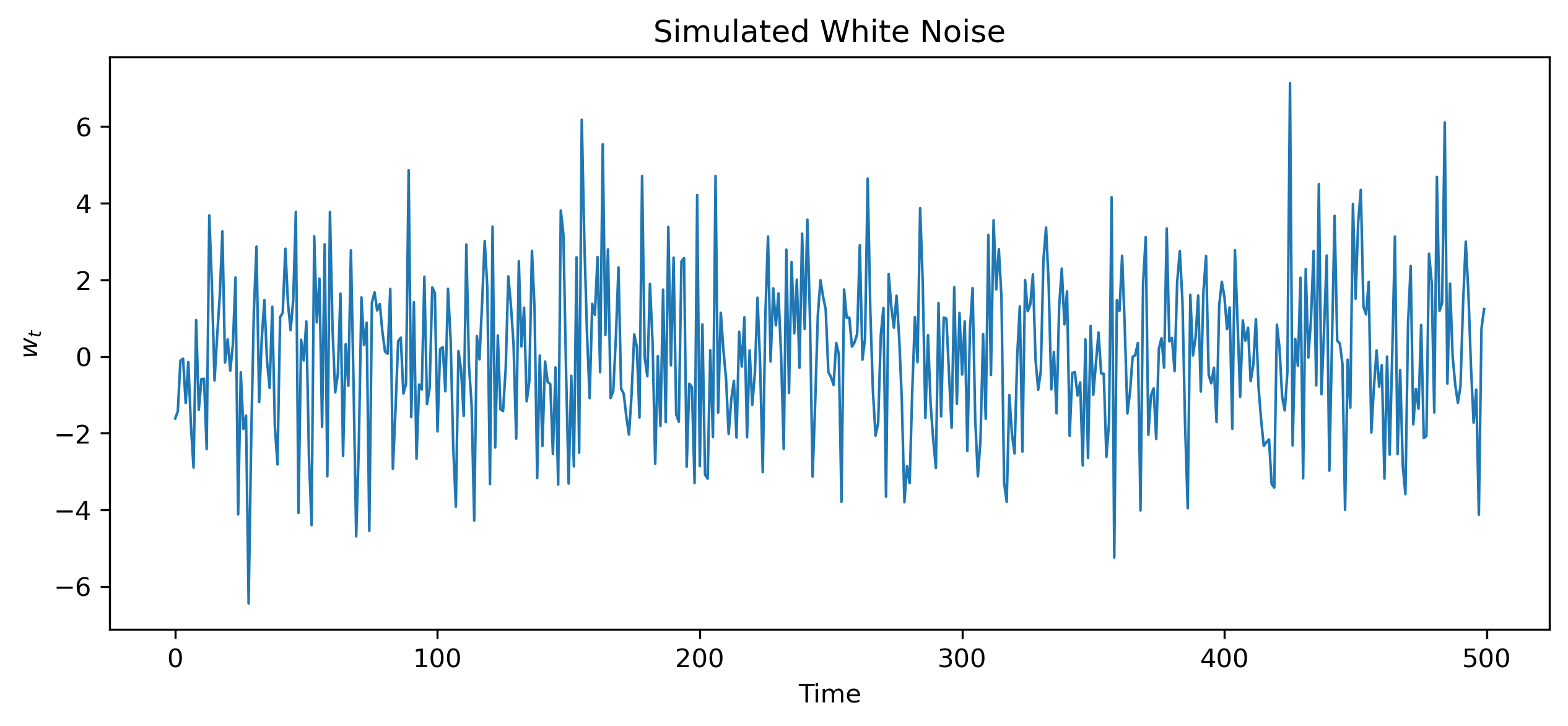

8.7 Random Walks Revisited¶

Now consider the random walk:

x_t = x_{t-1} + w_t

(5)

where $w_t$ is white noise.

Simulating a Random Walk¶

np.random.seed(123)

w = np.random.normal(0, 1, 500)
x = np.cumsum(w)

plt.figure(figsize=(10,4))
plt.plot(x, lw=1)
plt.title("Simulated Random Walk")
plt.xlabel("Time")
plt.ylabel("$x_t$")

# plt.savefig("figs/ch7/rw.png", dpi=300, bbox_inches="tight")
plt.close()   # replace with plt.show()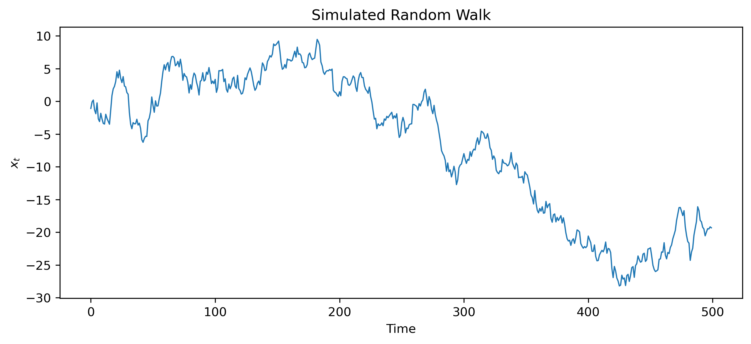

8.9 Why Random Walks Are Nonstationary¶

A random walk violates stationarity because:

shocks accumulate over time
variance grows continuously
no stable long-run mean exists

Variance of a Random Walk¶

Recall:

x_t = \sum_{s=1}^t w_s

Therefore:

Var(x_t) = t \sigma_w^2

This violates weak stationarity.

8.10 Stationary vs Nonstationary Series¶

Feature	Stationary	Nonstationary
Mean stable	Yes	Not necessarily
Variance stable	Yes	Often no
Dependence stable	Yes	Often no
Shocks temporary	Usually	Often persistent

8.11 Trend Stationary vs Difference Stationary¶

Not all nonstationary series behave in the same way.

Trend-Stationary Processes¶

Some series fluctuate around a deterministic trend:

x_t = \alpha + \beta t + u_t

(6)

where $u_t$ is stationary.

Removing the trend leaves a stationary process.

Difference-Stationary Processes¶

Other series become stationary only after differencing.

Random walks are the classic example.

8.12 Why Stationarity Matters for Forecasting¶

Forecasting relies heavily on stable patterns.

For stationary processes:

dependence structure is stable
past relationships remain informative

For nonstationary processes:

statistical properties evolve over time
prediction becomes more difficult

8.13 Why Stationarity Matters for Regression¶

Nonstationary variables can create misleading statistical relationships.

Two unrelated trending variables may appear strongly related.

This problem is called:

We study this in detail later in latter chapters.

8.14 Looking Ahead¶

In this chapter, we introduced the idea of stationarity and saw how random walks violate it.

In the next chapter, we study:

autocorrelation
autocovariance
partial autocorrelation

which help us understand dependence structures in stationary time series.

Key Takeaways¶

Concept Check¶

Basic¶

What is stationarity?
What does it mean for the mean of a series to be constant?
What does it mean for the variance to be constant?

Intuition¶

Why is stationarity important in time series analysis?
What happens if a series is not stationary?
Why are many financial price series not stationary?

Intermediate¶

What is the difference between:
- a stationary series
- a nonstationary series
What is mean reversion?
Why does a random walk violate stationarity?

Finance Insight¶

Why are returns often more stationary than prices?
Why is stationarity important for forecasting models?

Challenge¶

Suppose a series shows an upward trend but stable fluctuations around that trend.

Is this series stationary?
What transformation might help?

Interpretation & Practice¶

A time series fluctuates around a constant level with no visible trend.
- Is this likely stationary?
- Why?

A time series shows a steady upward trend.
- What does this suggest about stationarity?
- Why might this cause problems for modeling?

A series has increasing variability over time.
- What assumption of stationarity is violated?
- Why does this matter?

A random walk is plotted.
- Why does it appear to “wander” without returning to a fixed level?
- What does this imply about persistence?

A differenced series appears to fluctuate around zero.
- What does this suggest about stationarity?
- Why is differencing useful?

Finance Interpretation¶

A stock price series shows a strong upward trend.
- Why is this likely nonstationary?
- Why are returns preferred for modeling?

A return series appears stable over time.
- What does this suggest about stationarity?
- Why is this useful in practice?

Challenge¶

A model is estimated using nonstationary data.
- What kind of misleading results might occur?
- Why is this dangerous?

Numerical Practice¶

Identifying Stationarity¶

Consider the following series:
Series A:
2, −1, 1, −2, 0, 1, −1
Series B:
10, 12, 15, 18, 22, 27, 33

Which series appears stationary?
Which appears nonstationary?
Why?

Mean and Variance¶

Suppose a series behaves as follows:

First half: values fluctuate around 10
Second half: values fluctuate around 20

Is the mean constant?
Is the series stationary?

Suppose a series shows:

small fluctuations early
large fluctuations later

What property of stationarity is violated?

Differencing¶

Consider the series:
100, 102, 105, 109, 114

Compute the first differences
Does the differenced series appear more stable?

Suppose a random walk is defined as:

x_t = x_{t-1} + w_t

What would the differenced series look like?
Why is this important?

Challenge¶

Suppose a series has:

constant mean
constant variance
but strong dependence over time

Can it still be stationary?
Why?

Suppose you incorrectly treat a nonstationary series as stationary.

What type of errors might arise in modeling?