Part IV Capstone — Building and Evaluating ARIMA Models

In Part IV, we introduced the core linear models of time series analysis:

autoregressive (AR) models,
moving average (MA) models,
ARMA models,
and ARIMA models.

We learned how these models attempt to capture:

persistence,
dependence,
shocks,
and dynamic structure.

This capstone integrates these ideas through a practical forecasting workflow.

The emphasis is practical and intuition-first.

We focus on:

model identification,
estimation,
diagnostics,
and forecasting.

Learning Goals¶

By completing this capstone, you should be able to:

identify candidate ARIMA models
interpret ACF and PACF patterns
estimate AR, MA, ARMA, and ARIMA models
compare competing models
diagnose residuals
generate forecasts
evaluate forecasting performance visually

Dataset¶

We use the Gold price as the main example.

Exercise 1 — Download and Plot the Series¶

import yfinance as yf
import matplotlib.pyplot as plt

gold = yf.download(
    "GC=F",
    start="2023-01-01",
    auto_adjust=False
)

prices = gold["Adj Close"].squeeze()

prices.plot(figsize=(10,4))

plt.title("Gold")
plt.xlabel("Date")
plt.ylabel("USD")

plt.savefig("figs/ch14_/gold.png", dpi=300, bbox_inches="tight")
plt.close()   # replace with plt.show()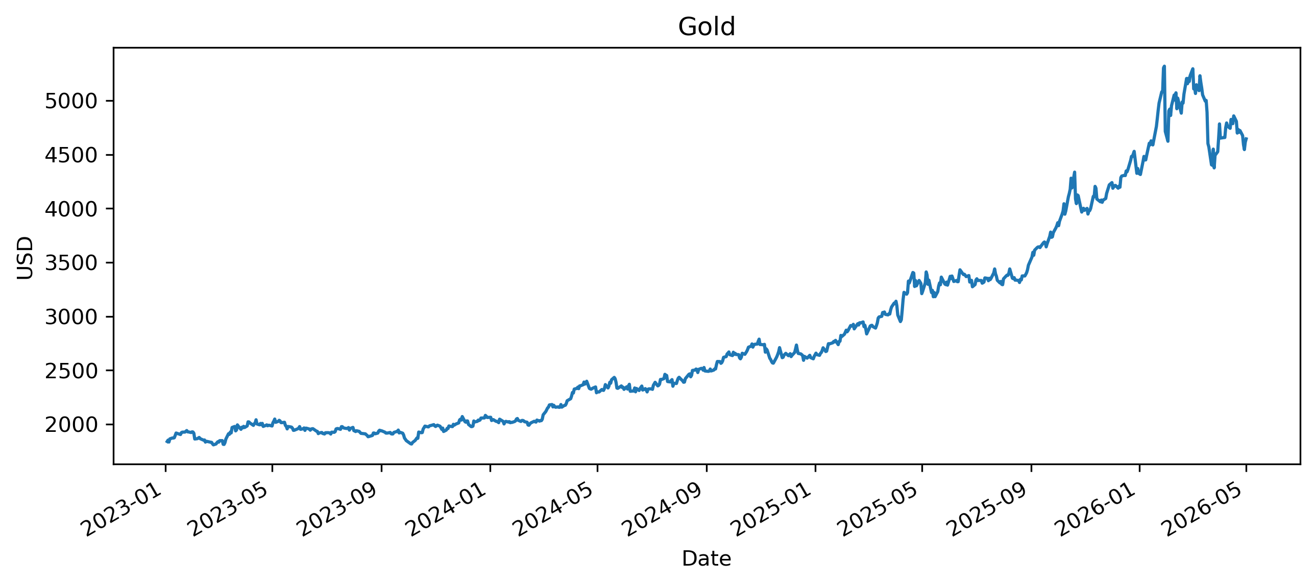

Questions¶

Does the series appear stationary?
Does it display trends or persistence?
Would ARIMA modeling likely require differencing?

Exercise 2 — Compute Log Returns¶

import numpy as np

returns = 100 * np.log(
    prices / prices.shift(1)
)

returns = returns.dropna()

returns.plot(figsize=(10,4))

plt.title("Gold Log Returns")
plt.xlabel("Date")
plt.ylabel("Return (%)")

plt.savefig("figs/ch14_/l_rtns.png", dpi=300, bbox_inches="tight")
plt.close()   # replace with plt.show()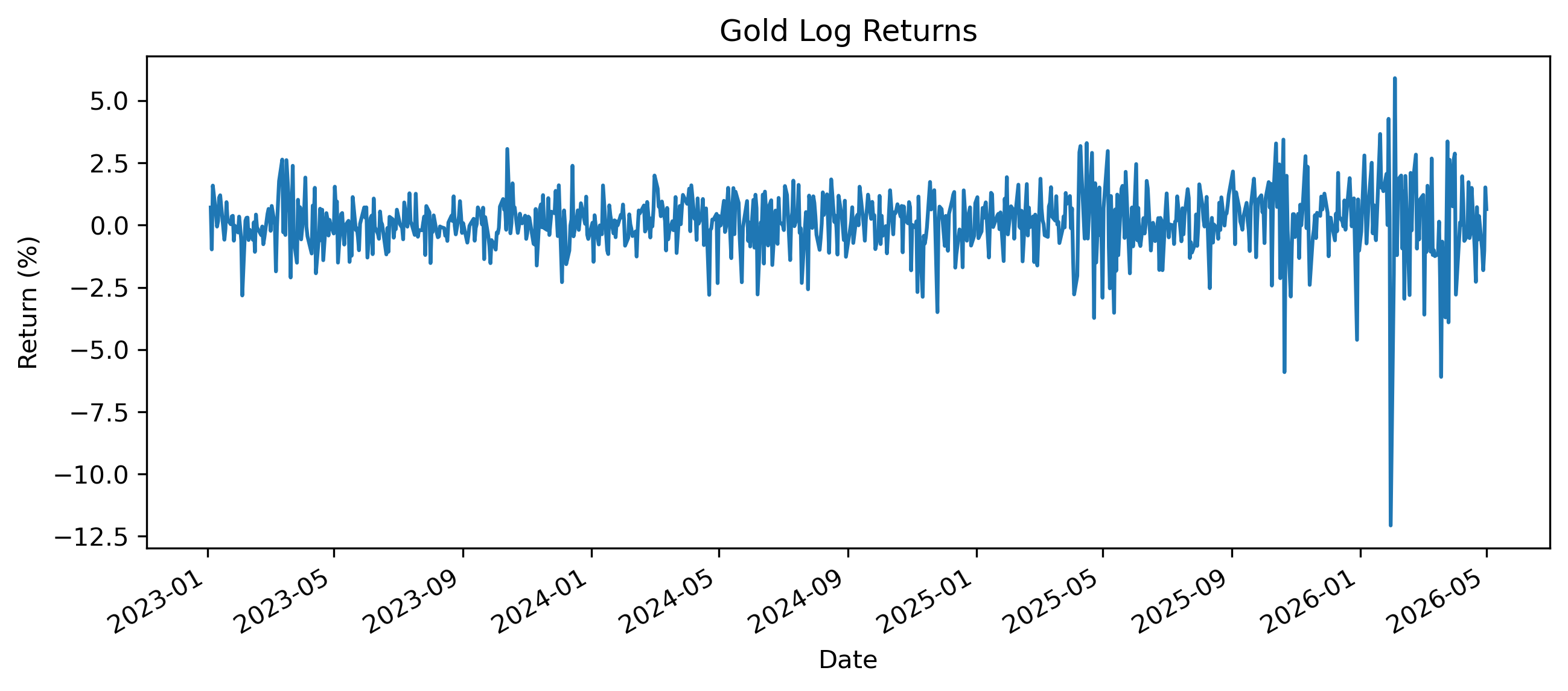

Exercise 3 — ACF and PACF¶

We now inspect autocorrelation patterns (ACF and PACF).

from statsmodels.graphics.tsaplots import (
    plot_acf,
    plot_pacf
)

# plot_acf(returns, lags=40)

# Plot ACF without lag 0
fig, ax = plt.subplots(1, 2, figsize=(10,4))
plot_acf(returns, lags=40, ax=ax[0])
ax[0].set_ylim(-0.15, 0.15)   # zoom y-axis
ax[0].set_xlim(0.5, 40)   # start at lag 1
ax[0].set_title("ACF (no lag 0)")

plot_pacf(returns, lags=40, ax=ax[1])
ax[1].set_ylim(-0.15, 0.15)   # zoom y-axis
ax[1].set_xlim(0.5, 40)   # start at lag 1
ax[1].set_title("PACF (no lag 0)")

plt.tight_layout()

plt.savefig("figs/ch14_/acf_pacf.png", dpi=300, bbox_inches="tight")
plt.close()   # replace with plt.show()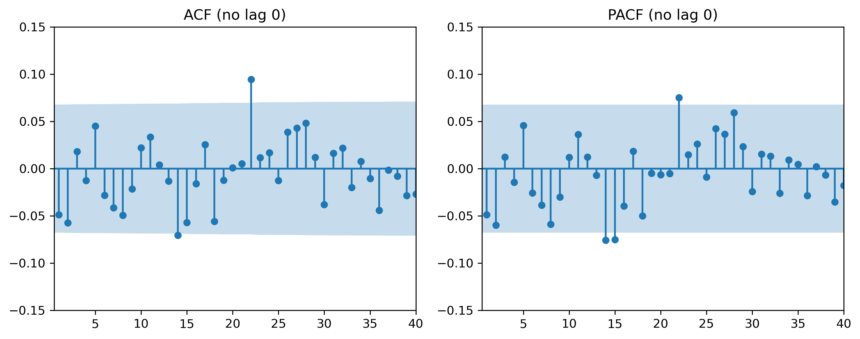

Questions¶

Do autocorrelations decay quickly?
Are there strong lag relationships?
Would an AR or MA model appear more appropriate?

Exercise 4 — Estimating an AR(2) Model¶

We begin with a simple autoregressive model.

from statsmodels.tsa.arima.model import ARIMA

ar2 = ARIMA(
    returns,
    order=(2,0,0)
).fit()

print(ar2.summary())

                               SARIMAX Results                                
==============================================================================
Dep. Variable:                   GC=F   No. Observations:                  836
Model:                 ARIMA(2, 0, 0)   Log Likelihood               -1363.339
Date:                Sat, 02 May 2026   AIC                           2734.678
Time:                        21:50:51   BIC                           2753.593
Sample:                             0   HQIC                          2741.929
                                - 836                                         
Covariance Type:                  opg                                         
==============================================================================
                 coef    std err          z      P>|z|      [0.025      0.975]
------------------------------------------------------------------------------
const          0.1103      0.042      2.636      0.008       0.028       0.192
ar.L1         -0.0519      0.026     -2.011      0.044      -0.103      -0.001
ar.L2         -0.0597      0.018     -3.284      0.001      -0.095      -0.024
sigma2         1.5276      0.034     44.552      0.000       1.460       1.595
===================================================================================
Ljung-Box (L1) (Q):                   0.00   Jarque-Bera (JB):              5453.72
Prob(Q):                              0.98   Prob(JB):                         0.00
Heteroskedasticity (H):               4.50   Skew:                            -1.42
Prob(H) (two-sided):                  0.00   Kurtosis:                        15.19
===================================================================================

Questions¶

Is the AR coefficient statistically significant?
Does the model imply persistence?
Are returns highly predictable?

Exercise 5 — Estimating an MA(2) Model¶

We now estimate a moving average model.

ma2 = ARIMA(
    returns,
    order=(0,0,2)
).fit()

print(ma2.summary())

                               SARIMAX Results                                
==============================================================================
Dep. Variable:                   GC=F   No. Observations:                  836
Model:                 ARIMA(0, 0, 2)   Log Likelihood               -1363.389
Date:                Sat, 02 May 2026   AIC                           2734.778
Time:                        21:50:51   BIC                           2753.693
Sample:                             0   HQIC                          2742.029
                                - 836                                         
Covariance Type:                  opg                                         
==============================================================================
                 coef    std err          z      P>|z|      [0.025      0.975]
------------------------------------------------------------------------------
const          0.1103      0.042      2.656      0.008       0.029       0.192
ma.L1         -0.0498      0.026     -1.920      0.055      -0.101       0.001
ma.L2         -0.0568      0.019     -3.063      0.002      -0.093      -0.020
sigma2         1.5278      0.035     44.006      0.000       1.460       1.596
===================================================================================
Ljung-Box (L1) (Q):                   0.00   Jarque-Bera (JB):              5439.20
Prob(Q):                              0.97   Prob(JB):                         0.00
Heteroskedasticity (H):               4.49   Skew:                            -1.41
Prob(H) (two-sided):                  0.00   Kurtosis:                        15.17
===================================================================================

Questions¶

Does the MA coefficient appear significant?
What economic interpretation might an MA structure have?
How does the MA model compare with the AR model?

Exercise 6 — Estimating an ARMA Model¶

We now estimate a combined ARMA(1,1) model.

arma11 = ARIMA(
    returns,
    order=(1,0,1)
).fit()

print(arma11.summary())

                               SARIMAX Results                                
==============================================================================
Dep. Variable:                   GC=F   No. Observations:                  836
Model:                 ARIMA(1, 0, 1)   Log Likelihood               -1363.662
Date:                Sat, 02 May 2026   AIC                           2735.323
Time:                        21:50:52   BIC                           2754.238
Sample:                             0   HQIC                          2742.574
                                - 836                                         
Covariance Type:                  opg                                         
==============================================================================
                 coef    std err          z      P>|z|      [0.025      0.975]
------------------------------------------------------------------------------
const          0.1106      0.036      3.083      0.002       0.040       0.181
ar.L1          0.8512      0.083     10.308      0.000       0.689       1.013
ma.L1         -0.8892      0.072    -12.278      0.000      -1.031      -0.747
sigma2         1.5287      0.036     42.797      0.000       1.459       1.599
===================================================================================
Ljung-Box (L1) (Q):                   0.19   Jarque-Bera (JB):              5217.36
Prob(Q):                              0.66   Prob(JB):                         0.00
Heteroskedasticity (H):               4.43   Skew:                            -1.34
Prob(H) (two-sided):                  0.00   Kurtosis:                        14.94
===================================================================================

Questions¶

Does the ARMA model fit better?
Which coefficients appear important?
Are the results economically meaningful?

Exercise 7 — Comparing AIC Values¶

We now compare model fit using information criteria.

print("AR(2) AIC:", ar2.aic)

print("MA(2) AIC:", ma2.aic)

print("ARMA(1,1) AIC:", arma11.aic)

AR(2) AIC: 2734.6781301831934
MA(2) AIC: 2734.77800194048
ARMA(1,1) AIC: 2735.3231523066397

Python has automatic lag selector:

import pandas as pd
import numpy as np
from statsmodels.tsa.statespace.sarimax import SARIMAX
from statsmodels.tsa.stattools import arma_order_select_ic

def fit_clean_arima(series, max_p=3, max_q=3):
    # 1. Ensure data is a 1D array (statsmodels is picky about DataFrames)
    data = series.values.flatten() if isinstance(series, (pd.DataFrame, pd.Series)) else series
    
    # 2. Automated Order Selection (Lower max_p/q to ensure it actually finishes)
    # We use AIC to find the best balance of complexity and fit
    print("Finding optimal orders... (this may take a moment)")
    res = arma_order_select_ic(data, max_ar=max_p, max_ma=max_q, ic='aic')
    p, q = res.aic_min_order
    
    # 3. Fit the model using SARIMAX (the modern version of ARIMA)
    # We set d=0 because returns are typically already stationary
    model = SARIMAX(data, order=(p, 0, q), enforce_stationarity=False, enforce_invertibility=False)
    results = model.fit(disp=False)
    
    print(f"Best Model Found: ARIMA({p}, 0, {q})")
    return results

# Usage
arma20 = fit_clean_arima(returns)
print(arma20.summary())

Best Model Found: ARIMA(2, 0, 0)
                               SARIMAX Results                                
==============================================================================
Dep. Variable:                      y   No. Observations:                  836
Model:               SARIMAX(2, 0, 0)   Log Likelihood               -1364.637
Date:                Sat, 02 May 2026   AIC                           2735.274
Time:                        22:00:50   BIC                           2749.452
Sample:                             0   HQIC                          2740.710
                                - 836                                         
Covariance Type:                  opg                                         
==============================================================================
                 coef    std err          z      P>|z|      [0.025      0.975]
------------------------------------------------------------------------------
ar.L1         -0.0425      0.027     -1.592      0.111      -0.095       0.010
ar.L2         -0.0508      0.018     -2.807      0.005      -0.086      -0.015
sigma2         1.5444      0.033     46.489      0.000       1.479       1.610
===================================================================================
Ljung-Box (L1) (Q):                   0.04   Jarque-Bera (JB):              5569.40
Prob(Q):                              0.84   Prob(JB):                         0.00
Heteroskedasticity (H):               4.62   Skew:                            -1.42
Prob(H) (two-sided):                  0.00   Kurtosis:                        15.33
===================================================================================

Questions¶

Which model has the lowest AIC?
Why do we penalize model complexity?
Does the best statistical model necessarily produce the best forecasts?

Exercise 8 — Residual Diagnostics¶

A good model should leave residuals resembling white noise.

import pandas as pd
import matplotlib.pyplot as plt

residuals = pd.Series(
    arma20.resid,
    index=returns.index[-len(arma20.resid):]
)

residuals.plot(figsize=(10,4))

plt.title("Residuals from AR(2) Model")

plt.savefig("figs/ch14_/res.png", dpi=300, bbox_inches="tight")
plt.close()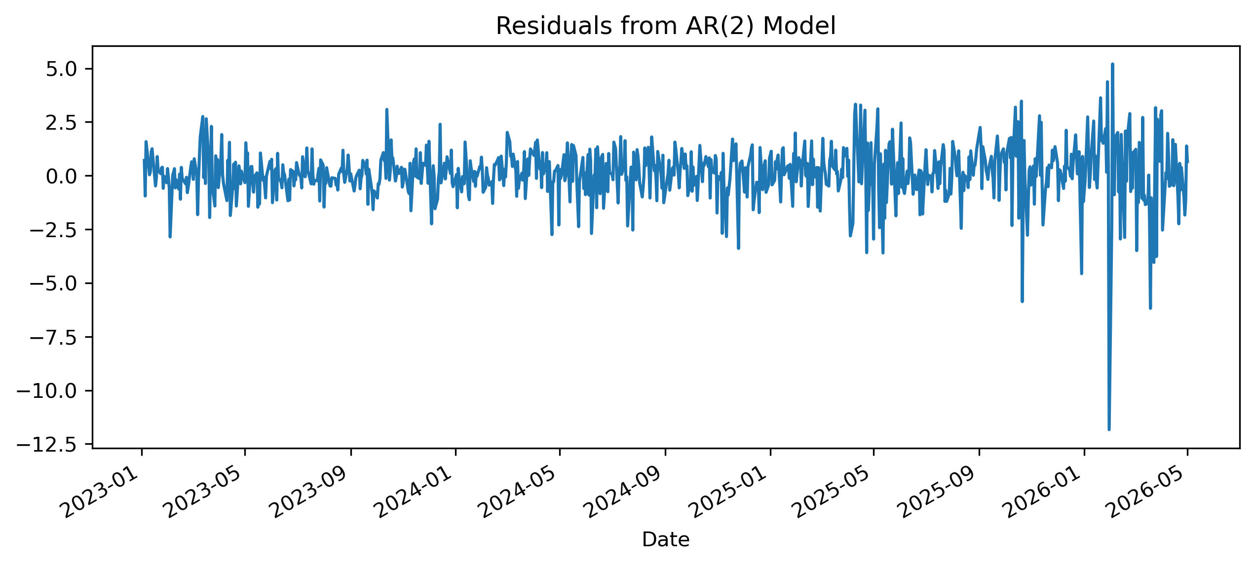

Exercise 9 — Residual ACF¶

plot_acf(
    residuals,
    lags=40
)

plt.title("ACF of Residuals")

plt.show()

Questions¶

Do residual autocorrelations remain?
Does the model adequately capture dependence?
Why is residual whiteness important?

Exercise 10 — Ljung-Box Test¶

We now formally test residual autocorrelation.

from statsmodels.stats.diagnostic import acorr_ljungbox

acorr_ljungbox(
    residuals,
    lags=[10],
    return_df=True
)

Questions¶

What is the null hypothesis?
Is there evidence of remaining autocorrelation?
What would strong residual autocorrelation imply?

Exercise 11 — Forecasting¶

We now generate forecasts.

# 1. Fit the model using the function we defined
results = fit_clean_arima(returns)

# 2. Generate the forecast
n_steps = 20
forecast_obj = results.get_forecast(steps=n_steps)

# Extract predicted mean and confidence intervals
mean = forecast_obj.predicted_mean
conf_int = forecast_obj.conf_int()

# 3. Plotting
plt.figure(figsize=(10, 5))

# Plot the last 100 actual observations
plt.plot(returns.index[-100:], returns[-100:], label="Observed", color='black', alpha=0.6)

# Plot the forecast
# Note: SARIMAX usually handles the index automatically if 'returns' was a Pandas Series
plt.plot(mean.index, mean, label="Forecast", color='crimson', lw=2)

# Shade the confidence interval
plt.fill_between(
    conf_int.index, 
    conf_int.iloc[:, 0], 
    conf_int.iloc[:, 1], 
    color='crimson', 
    alpha=0.15, 
    label="95% Confidence Interval"
)

plt.title("ARIMA Forecast: Future Returns")
plt.legend(loc='upper left')
plt.grid(axis='y', alpha=0.3)
plt.show()

Exercise 12 — ARIMA for Nonstationary Data¶

Suppose we model price levels directly instead of returns.

We now estimate an ARIMA model with differencing.

arima111 = ARIMA(
    prices,
    order=(1,1,1)
).fit()

print(arima111.summary())

Questions¶

Why is differencing required here?
What does the integrated component represent?
How does ARIMA differ from ARMA?

Exercise 13 — Comparing Forecasts¶

We now compare forecasts from:

ARMA on returns,
ARIMA on prices.

Questions¶

Which approach appears more stable?
Which series is easier to forecast?
Why are financial returns often difficult to predict?

Exercise 14 — Simulating an AR(1) Process¶

We now simulate a known AR(1) process.

import numpy as np

np.random.seed(123)

T = 300

phi = 0.7

e = np.random.normal(size=T)

x = np.zeros(T)

for t in range(1, T):
    x[t] = phi * x[t-1] + e[t]

plt.figure(figsize=(10,4))

plt.plot(x)

plt.title("Simulated AR(1) Process")

plt.show()

Questions¶

Does the series appear persistent?
Does it look stationary?
How does it compare with real financial returns?

Exercise 15 — Simulating a Random Walk¶

np.random.seed(123)

e = np.random.normal(size=T)

rw = np.cumsum(e)

plt.figure(figsize=(10,4))

plt.plot(rw)

plt.title("Simulated Random Walk")

plt.show()

Questions¶

Does the random walk resemble the SET price level?
Why is a random walk difficult to forecast?
How does differencing affect the random walk?

Mini Project — Building Your Own Forecasting Model¶

Choose one time series.

Examples:

SET Index,
exchange rate,
CPI,
gold prices,
oil prices,
Bitcoin,
interest rates.

Complete the following tasks:

Plot the series.
Test for stationarity.
Difference if necessary.
Plot ACF and PACF.
Estimate several ARIMA-type models.
Compare AIC values.
Diagnose residuals.
Generate forecasts.
Interpret forecasting performance.

Gretl Version¶

The same workflow can be implemented in GRETL.

Estimating ARIMA Models¶

Menu:

Model → Time Series → ARIMA

Residual Diagnostics¶

Menu:

Tests → Autocorrelation

Forecasting¶

Menu:

Analysis → Forecasts

[GRETL Screenshot Placeholder: ARIMA estimation output]

Common Mistakes¶

Looking Ahead¶

Part V focuses explicitly on forecasting.

We now move beyond:

estimating models,

toward:

evaluating forecast quality,
comparing forecasting methods,
and measuring forecast performance.

Part IV Capstone — Building and Evaluating ARIMA Models

Learning Goals¶

Dataset¶

Exercise 1 — Download and Plot the Series¶

Questions¶

Exercise 2 — Compute Log Returns¶

Exercise 3 — ACF and PACF¶

Questions¶

Exercise 4 — Estimating an AR(2) Model¶

Questions¶

Exercise 5 — Estimating an MA(2) Model¶

Questions¶

Exercise 6 — Estimating an ARMA Model¶

Questions¶

Exercise 7 — Comparing AIC Values¶

Questions¶

Exercise 8 — Residual Diagnostics¶

Exercise 9 — Residual ACF¶

Questions¶

Exercise 10 — Ljung-Box Test¶

Questions¶

Exercise 11 — Forecasting¶

Exercise 12 — ARIMA for Nonstationary Data¶

Questions¶

Exercise 13 — Comparing Forecasts¶

Questions¶

Exercise 14 — Simulating an AR(1) Process¶

Questions¶

Exercise 15 — Simulating a Random Walk¶

Questions¶

Mini Project — Building Your Own Forecasting Model¶

Gretl Version¶

Estimating ARIMA Models¶

Residual Diagnostics¶

Forecasting¶

Common Mistakes¶

Looking Ahead¶

Key Takeaways¶