Chapter 9 — ACF and PACF - Applied Time Series

In previous chapters, we introduced dependence, persistence, and stationarity.

We now develop two of the most important tools in time series analysis:

the autocorrelation function (ACF)
the partial autocorrelation function (PACF)

These tools help us understand:

dependence across time
persistence
lag structure
model identification

Learning Objectives¶

By the end of this chapter, you should be able to:

understand autocorrelation and autocovariance
interpret ACF and PACF plots
recognize dependence patterns
distinguish white noise and persistent processes
use ACF/PACF for model identification

9.1 Correlation Across Time¶

In time series analysis, we study relationships such as:

Corr(X_t, X_{t-h})

where (h) is the lag.

9.2 Autocovariance and ACF¶

For a weakly stationary process:

\gamma(h) = Cov(X_t, X_{t-h})

The autocorrelation function (ACF) is:

\rho(h) = \frac{\gamma(h)}{\gamma(0)}

where (\gamma(0) = Var(X_t)).

9.3 White Noise: No Dependence¶

Simulation¶

import numpy as np
import matplotlib.pyplot as plt
from statsmodels.graphics.tsaplots import plot_acf, plot_pacf

np.random.seed(10101)

wn = np.random.normal(0, 1, 300)

plt.figure(figsize=(10,4))
plt.plot(wn)
plt.title("White Noise")
plt.savefig("figs/ch9/wn.png", dpi=300, bbox_inches="tight")
plt.close()   # replace with plt.show()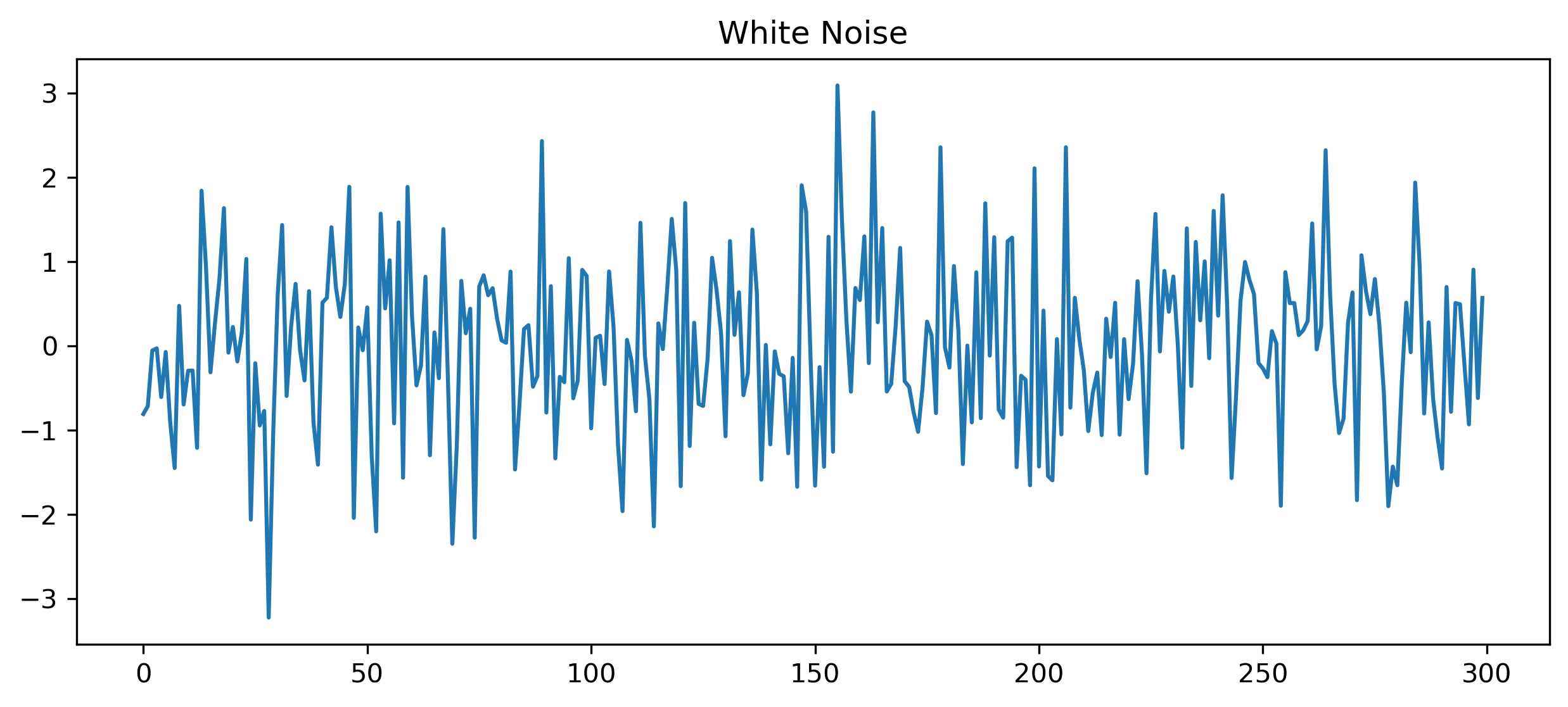

ACF and PACF¶

fig, ax = plt.subplots(1,2, figsize=(10,4))

plot_acf(wn, lags=30, ax=ax[0])
ax[0].set_title("ACF (White Noise)")

plot_pacf(wn, lags=30, ax=ax[1], method="ywm")
ax[1].set_title("PACF (White Noise)")

plt.savefig("figs/ch9/wn_acf_pacf.png", dpi=300, bbox_inches="tight")
plt.close()   # replace with plt.show()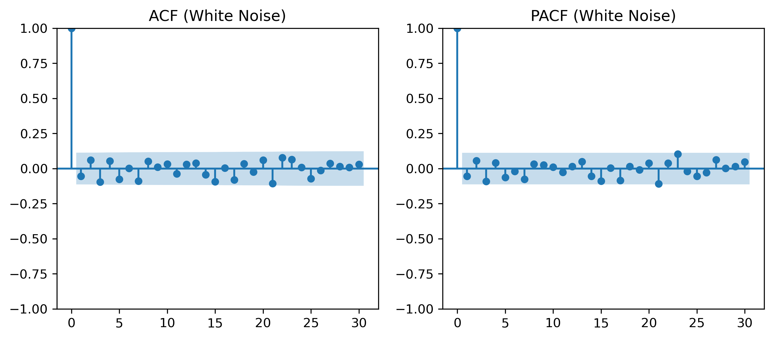

9.4 Persistent Series: Random Walk¶

Simulation¶

np.random.seed(123)

w = np.random.normal(0, 1, 300)
x = np.cumsum(w)

plt.figure(figsize=(10,4))
plt.plot(x)
plt.title("Random Walk")

plt.savefig("figs/ch9/rw.png", dpi=300, bbox_inches="tight")
plt.close()   # replace with plt.show()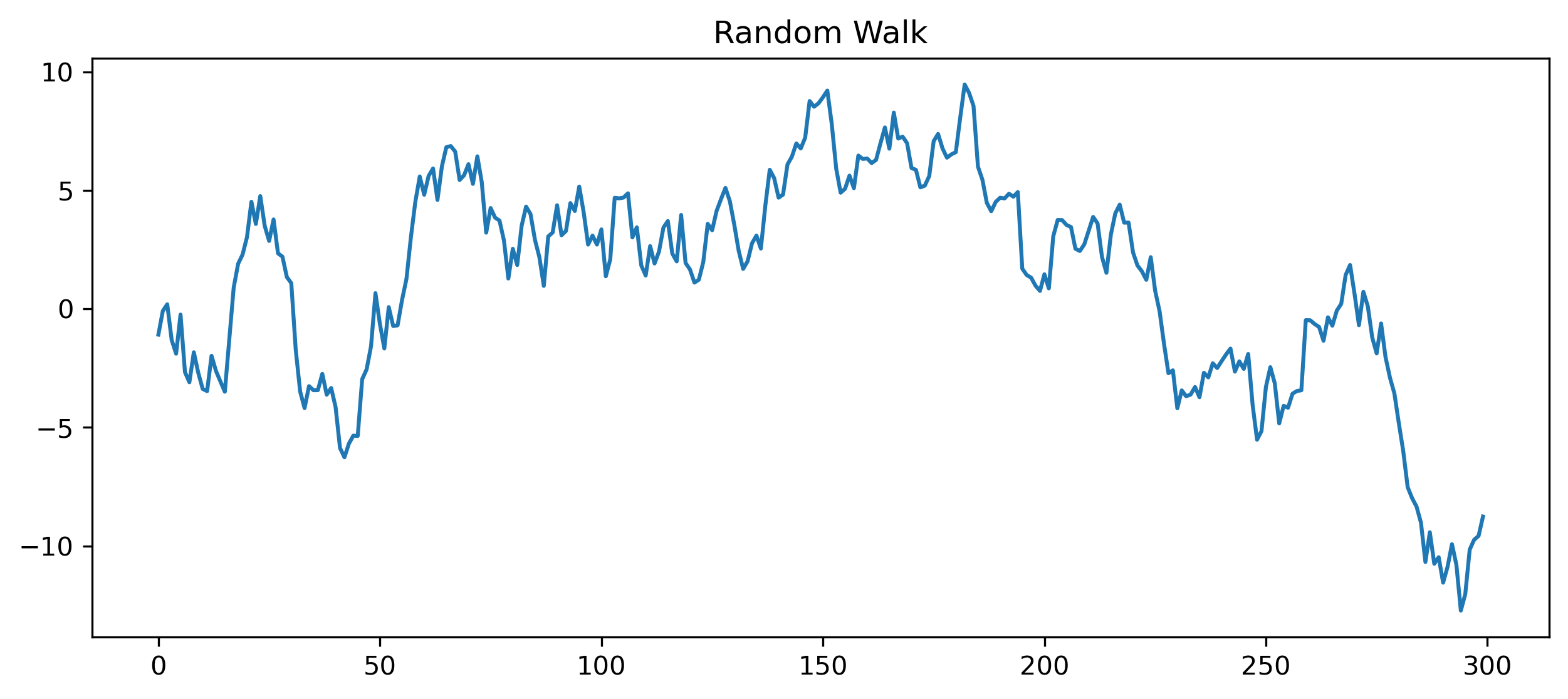

ACF and PACF¶

fig, ax = plt.subplots(1,2, figsize=(10,4))

plot_acf(x, lags=40, ax=ax[0])
ax[0].set_title("ACF (Random Walk)")

plot_pacf(x, lags=40, ax=ax[1], method="ywm")
ax[1].set_title("PACF (Random Walk)")

plt.tight_layout()

plt.savefig("figs/ch9/rw_acf_pacf.png", dpi=300, bbox_inches="tight")
plt.close()   # replace with plt.show()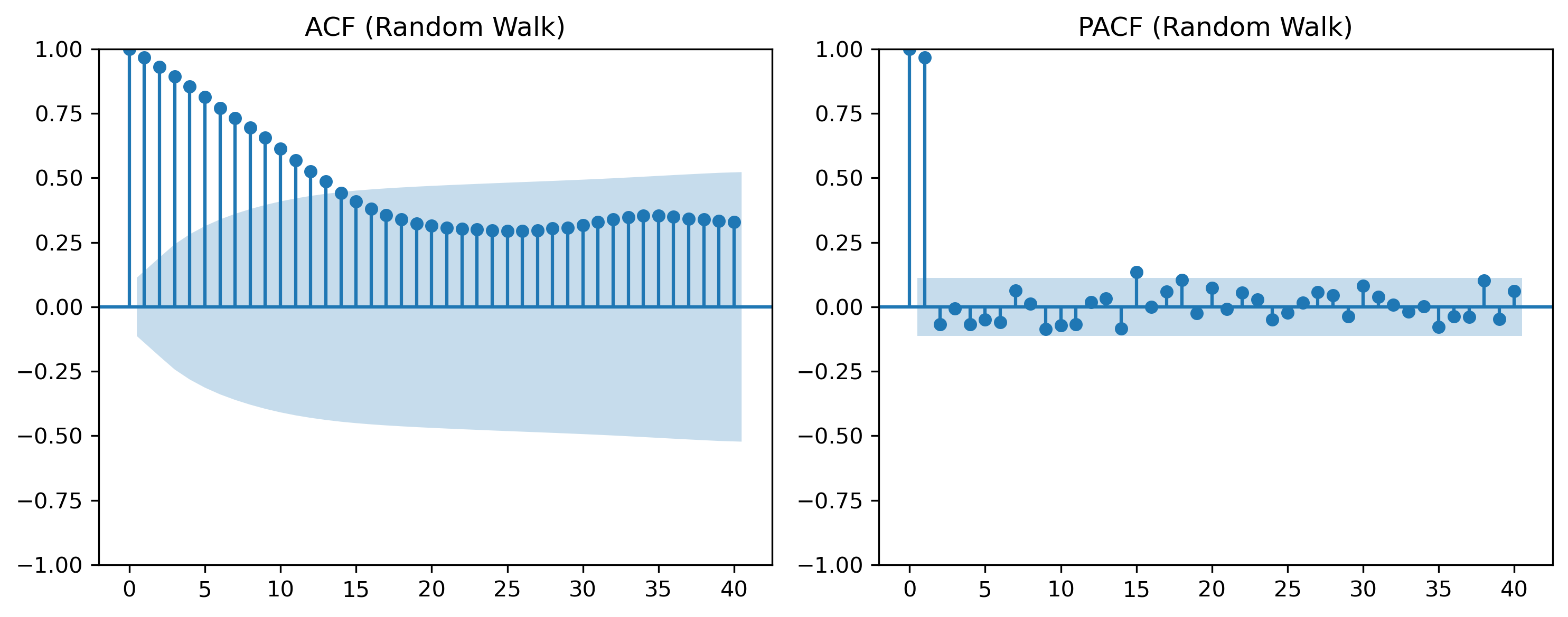

9.5 Interpreting ACF Patterns¶

White Noise¶

ACF ≈ 0 at all lags

Persistent Series¶

ACF decays slowly

Oscillatory Behavior¶

ACF alternates signs

9.6 Partial Autocorrelation (PACF)¶

The ACF measures total dependence, including indirect effects.

The PACF isolates direct dependence.

9.7 ACF vs PACF (Intuition)¶

9.8 Visual Comparison¶

np.random.seed(42)

# AR(1)
phi = 0.7
ar = np.zeros(300)

for t in range(1, 300):
    ar[t] = phi * ar[t-1] + np.random.normal()

fig, ax = plt.subplots(2,2, figsize=(10,6))

plot_acf(ar, lags=30, ax=ax[0,0])
ax[0,0].set_title("ACF (AR(1))")

plot_pacf(ar, lags=30, ax=ax[0,1], method="ywm")
ax[0,1].set_title("PACF (AR(1))")

plot_acf(wn, lags=30, ax=ax[1,0])
ax[1,0].set_title("ACF (White Noise)")

plot_pacf(wn, lags=30, ax=ax[1,1], method="ywm")
ax[1,1].set_title("PACF (White Noise)")

plt.tight_layout()

plt.savefig("figs/ch9/acf_pacf_.png", dpi=300, bbox_inches="tight")
plt.close()   # replace with plt.show()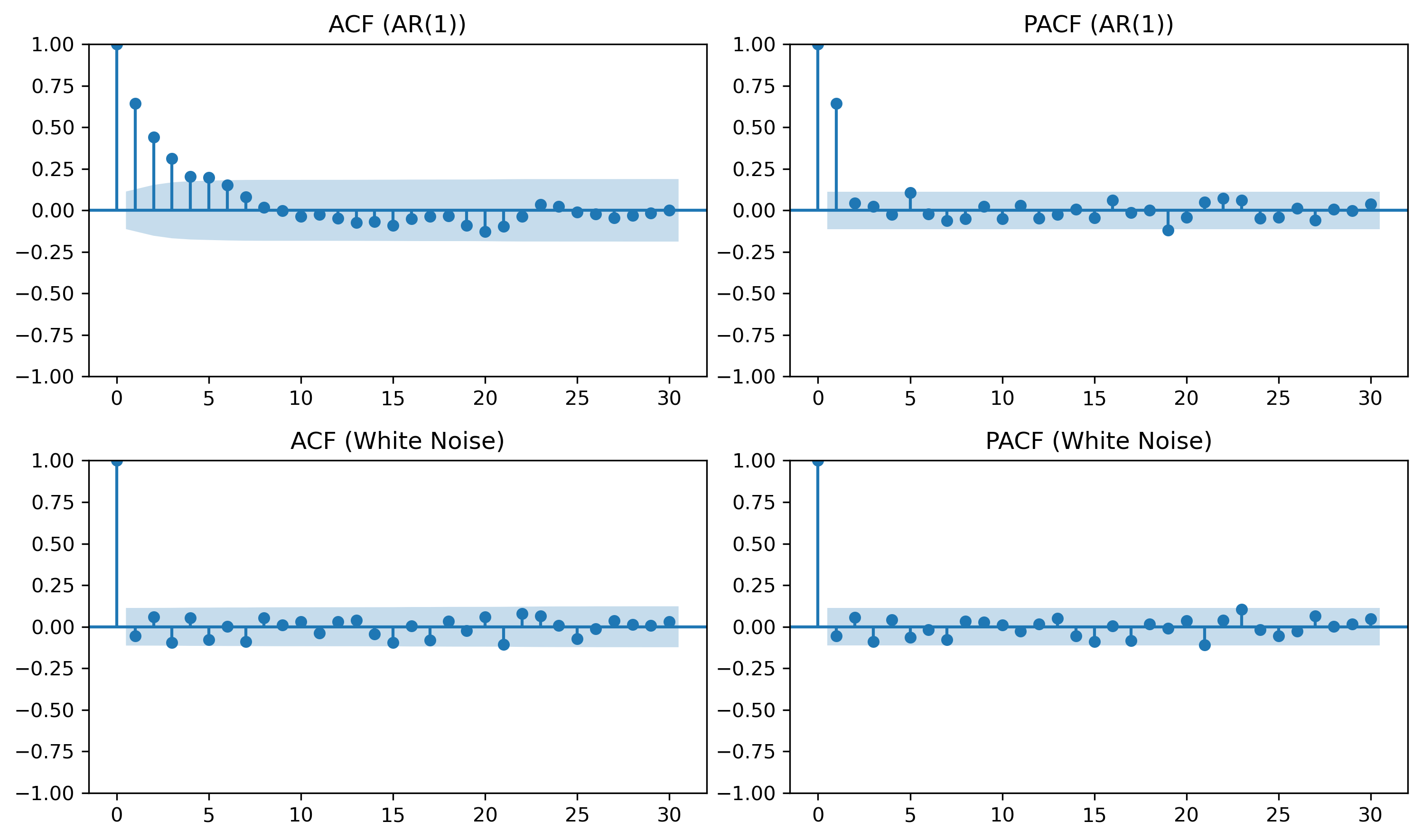

9.9 Model Identification (Rule of Thumb)¶

Model	ACF	PACF
AR(p)	decays	cuts off at p
MA(q)	cuts off at q	decays
ARMA	decays	decays
White noise	none	none

9.10 Confidence Bands¶

ACF/PACF plots include approximate bounds:

\pm \frac{2}{\sqrt{T}}

9.11 Economic and Financial Insight¶

Macroeconomic variables → persistent
Financial returns → weak autocorrelation
Volatility → highly persistent

9.12 Looking Ahead¶

ACF and PACF help diagnose dependence patterns.

Next, we study:

unit roots
nonstationarity
differencing

which explain whether persistence is temporary or permanent.

Key Takeaways¶

Concept Check¶

Basic¶

What is autocorrelation?
What does the autocorrelation function (ACF) measure?
What is a lag?

Intuition¶

Why do we examine correlations across time in a time series?
What does a high autocorrelation at lag 1 suggest?
What does it mean if autocorrelations decay slowly?

Intermediate¶

What is the difference between:
- ACF
- PACF
Why is PACF useful in time series analysis?
What does it mean if autocorrelations are close to zero at all lags?

Interpretation¶

What pattern would you expect in the ACF of:

white noise
a persistent series

Challenge¶

Suppose the ACF shows strong values at many lags.

What does this suggest about the series?
Why might this indicate nonstationarity?

Interpretation & Practice¶

ACF values are close to zero at all lags.
- What type of process is this likely?
- Why?
ACF shows a large value at lag 1, then quickly drops to zero.
- What does this suggest about dependence?
- What type of process might generate this?
ACF decays slowly over many lags.
- What does this indicate?
- Why might this suggest nonstationarity?
PACF shows a sharp cutoff after lag 1.
- What does this imply?
- Why is this useful for model identification?
ACF alternates between positive and negative values.
- What type of behavior might this indicate?
- What does this suggest about the series dynamics?

Finance Interpretation¶

A return series shows very low autocorrelation.
- What does this imply about predictability?
- How does this relate to market efficiency?
A volatility series shows strong autocorrelation.
- What does this suggest?
- Why is this important in finance?

Challenge¶

Suppose both ACF and PACF show no clear pattern.
- What type of process might this be?
- Why is model identification difficult in this case?

Numerical Practice¶

Identifying Autocorrelation¶

Consider the following series:
2, 4, 6, 8, 10

Does this series show dependence over time?
Would you expect high autocorrelation?
Why?

Consider:
3, −1, 2, −2, 1, 0

Does this series appear random?
Would you expect autocorrelation to be high or low?

Lag Interpretation¶

Suppose:

Corr(X_t, X_{t-1}) = 0.8

What does this imply?
Is the series highly dependent?

Suppose:

Corr(X_t, X_{t-1}) \approx 0

What does this suggest about predictability?

ACF Patterns¶

Match the pattern:

ACF ≈ 0 for all lags
ACF slowly decays
ACF cuts off quickly

To the likely process:

white noise
persistent series
short-memory process

Challenge¶

Suppose a series has:

strong autocorrelation at lag 1
weak autocorrelation afterward

What type of model might describe this?
Why?

Appendix 9A — Understanding PACF¶

The PACF can be interpreted as the correlation between:

$X_t$
and $X_{t-h}$

after removing the effect of intermediate lags.

This can be obtained by:

Regressing $X_t$ on intermediate lags
Regressing $X_{t-h}$ on the same variables
Taking the correlation between residuals