Chapter 14 — ARIMA Models - Applied Time Series

In the previous chapters, we studied:

autoregressive (AR) models
moving average (MA) models
ARMA models

These models assume that the underlying process is stationary.

However, many economic and financial time series are not stationary.

Examples include:

stock prices
GDP
exchange rates
price indices

These series often exhibit:

trends
persistent drift
unit roots

The solution is to transform the data before modeling.

Learning Objectives¶

By the end of this chapter, you should be able to:

understand the motivation behind ARIMA models
distinguish stationary and integrated processes
understand the role of differencing
define ARIMA( $p,d,q$ ) models
interpret the Box–Jenkins workflow
estimate ARIMA models in Gretl
evaluate residual diagnostics and model fit

14.1 Why ARIMA Models?¶

Many real-world time series exhibit strong persistence and nonstationarity.

For example:

stock prices drift over time
GDP tends to grow
inflation may exhibit persistent trends

Applying stationary ARMA models directly to such data may produce misleading results.

14.2 Differencing Revisited¶

Recall the first difference operator:

\Delta x_t = x_t - x_{t-1}

Differencing removes persistent stochastic trends.

Example: Random Walk¶

Suppose:

x_t = x_{t-1} + w_t

Then:

\Delta x_t = w_t

which is white noise.

14.3 Integrated Processes¶

First Difference¶

\Delta x_t = x_t - x_{t-1}

Second Difference¶

\Delta^2 x_t = \Delta(\Delta x_t)

or:

\Delta^2 x_t = x_t - 2x_{t-1} + x_{t-2}

14.4 The ARIMA Model¶

General Form¶

After differencing $d$ times:

\phi(B)(1-B)^d x_t = \theta(B)w_t

(1)

where:

$\phi(B)$ is the AR polynomial
$(1-B)^d$ is the differencing operator
$\theta(B)$ is the MA polynomial

14.5 Understanding the Components¶

AR Component¶

Captures persistence through past values.

I Component¶

Captures nonstationarity through differencing.

MA Component¶

Captures temporary propagation of shocks.

14.6 Example: ARIMA(0,1,0)¶

Consider:

(1-B)x_t = w_t

or:

x_t - x_{t-1} = w_t

Thus:

x_t = x_{t-1} + w_t

14.7 Example: ARIMA(1,1,0)¶

Suppose:

(1-\phi B)(1-B)x_t = w_t

or equivalently:

\Delta x_t = \phi \Delta x_{t-1} + w_t

14.8 Example: ARIMA(0,1,1)¶

Suppose:

(1-B)x_t = (1+\theta B)w_t

Then:

\Delta x_t = w_t + \theta w_{t-1}

14.9 Simulating an ARIMA Process¶

import numpy as np
import matplotlib.pyplot as plt

np.random.seed(123)

n = 400

phi = 0.7

w = np.random.normal(size=n)

dx = np.zeros(n)

for t in range(1,n):
    dx[t] = phi*dx[t-1] + w[t]

x = np.cumsum(dx)

fig, ax = plt.subplots(2,1, figsize=(10,6))

ax[0].plot(dx)
ax[0].set_title("Differenced Series")

ax[1].plot(x)
ax[1].set_title("Integrated Series")

plt.tight_layout()

plt.savefig("figs/ch14/ARIMA.png", dpi=300, bbox_inches="tight")
plt.close()   # replace with plt.show()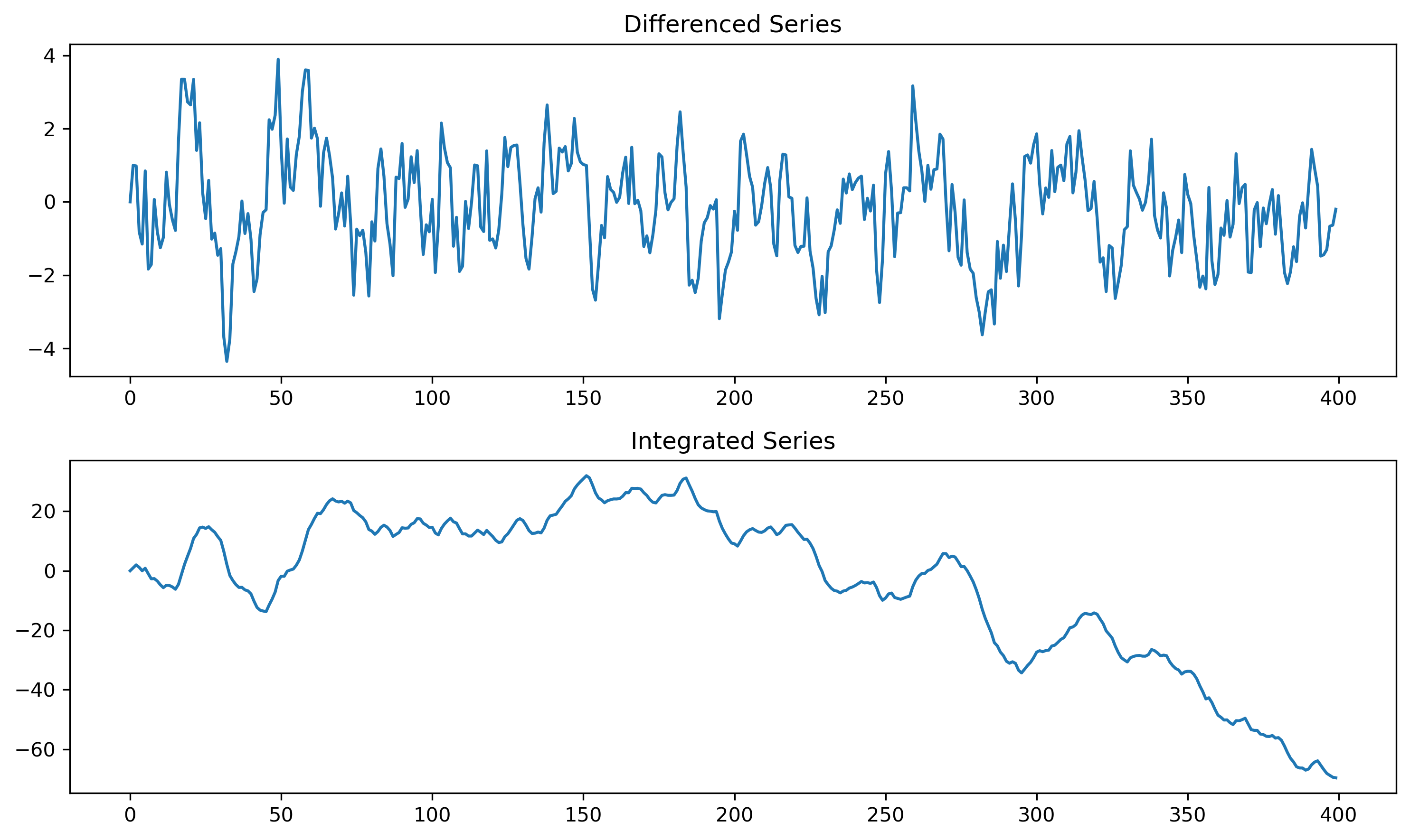

14.10 The Box–Jenkins Methodology¶

Classical ARIMA modeling follows the Box–Jenkins approach.

Step 1 — Identification¶

plot the data
check stationarity
difference if necessary
examine ACF/PACF

Step 2 — Estimation¶

Estimate candidate ARIMA models.

Step 3 — Diagnostic Checking¶

Check whether residuals resemble white noise.

Step 4 — Forecasting¶

Generate forecasts and evaluate performance.

14.11 Identifying Differencing Order¶

A series may require differencing if:

it exhibits persistent trends
ACF decays very slowly
unit root tests fail to reject nonstationarity

14.12 Under-Differencing vs Over-Differencing¶

Under-Differencing¶

residual nonstationarity remains
strong persistence persists

Over-Differencing¶

introduces excess noise
may create artificial negative autocorrelation

14.13 ACF and PACF in ARIMA Modeling¶

After differencing:

examine ACF
examine PACF
identify possible AR and MA orders

Typical Patterns¶

Model	ACF	PACF
AR( $p$ )	tails off	cuts off
MA( $q$ )	cuts off	tails off
ARMA( $p,q$ )	tails off	tails off

14.14 Estimation in Gretl¶

Model → Time Series → ARIMA

Typical Workflow¶

plot the series
test for unit roots
difference if needed
inspect ACF/PACF
estimate candidate models
compare AIC/BIC
check residuals

[GRETL Screenshot Placeholder: ARIMA estimation dialog]

[GRETL Screenshot Placeholder: ARIMA output]

14.15 Residual Diagnostics¶

Residuals should resemble white noise.

Residual ACF¶

import statsmodels.api as sm
from statsmodels.graphics.tsaplots import plot_acf

model = sm.tsa.ARIMA(x, order=(1,1,0))
res = model.fit()

plot_acf(res.resid, lags=20)

plt.savefig("figs/ch14/acf.png", dpi=300, bbox_inches="tight")
plt.close()   # replace with plt.show()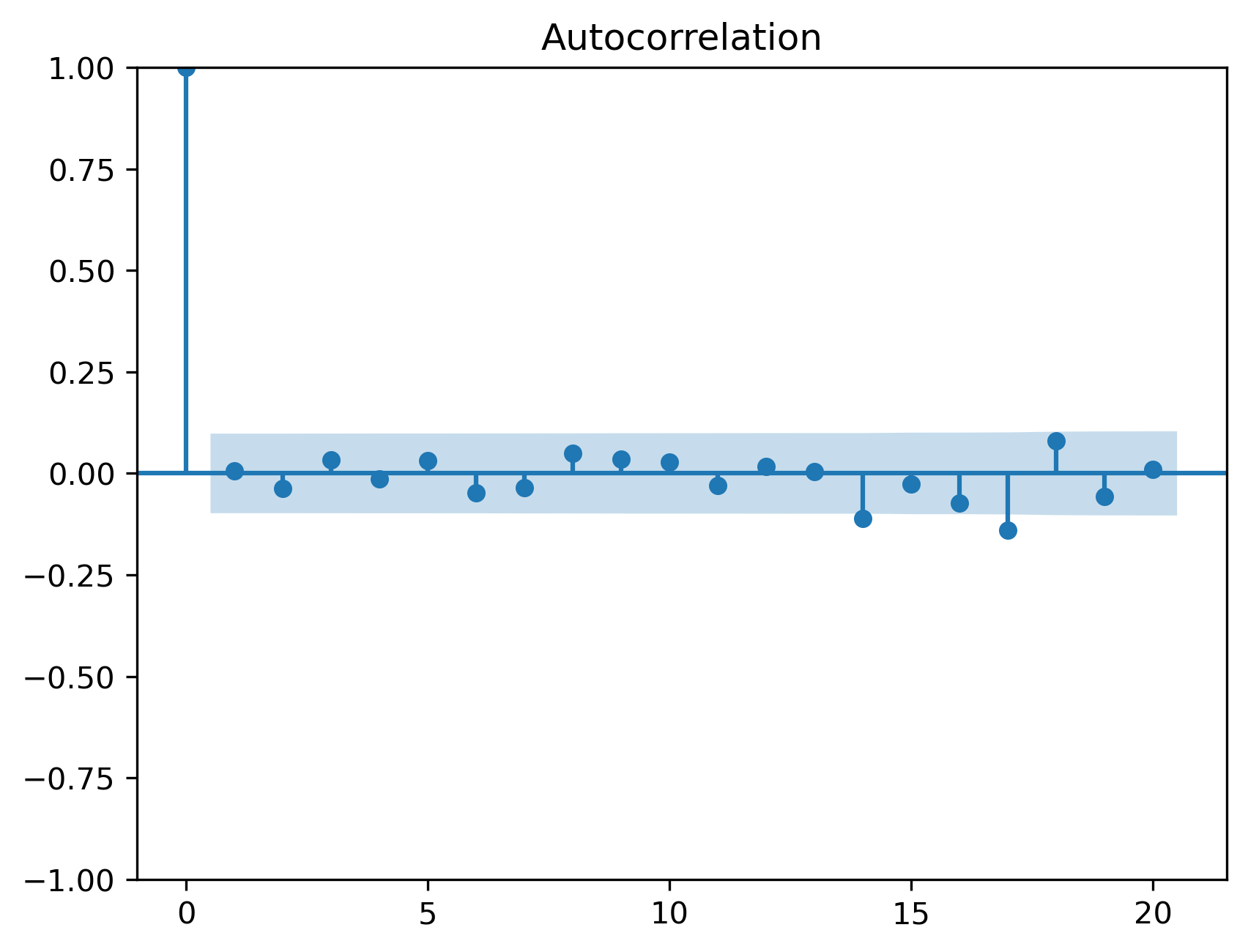

Ljung–Box Test¶

from statsmodels.stats.diagnostic import acorr_ljungbox

acorr_ljungbox(res.resid, lags=[10,20], return_df=True)

|  | lb_stat   | lb_pvalue |
|---------|------------|-----------|
| 10      | 4.729113   | 0.908524  |
| 20      | 25.169131  | 0.195037  |

14.16 Information Criteria¶

Model selection often uses:

Akaike Information Criterion¶

AIC = -2\log(\hat L) + 2k

(2)

Bayesian Information Criterion¶

BIC = -2\log(\hat L) + k\log n

(3)

14.17 Forecasting with ARIMA Models¶

Once estimated, ARIMA models can generate forecasts.

Multi-Step Forecasts¶

Forecasts are generated recursively using:

past observations
estimated parameters
projected future dynamics

14.18 ARIMA Models in Economics and Finance¶

ARIMA models are widely used for:

GDP forecasting
inflation forecasting
demand forecasting
exchange rates
inventory management
energy consumption

14.19 Common Mistakes¶

14.20 Looking Ahead¶

In this chapter, we extended ARMA models to handle nonstationary series through differencing.

We now move to forecasting and forecast evaluation, where we study:

static vs dynamic forecasting
forecast accuracy
RMSE, MAE, MAPE
Theil’s U statistics

Key Takeaways¶

Concept Check¶

Basic¶

What is an ARIMA model?
What does the “I” in ARIMA represent?
What does differencing do to a time series?

Intuition¶

Why are many economic time series nonstationary?
Why is it problematic to apply ARMA models to nonstationary data?
What is the idea behind transforming data before modeling?

Intermediate¶

What does it mean for a series to be:
- $I(0)$
- $I(1)$
What is the difference between first and second differencing?
Why is most real-world data $I(1)$ rather than $I(2)$ ?

ARIMA Structure¶

What do $p$ , $d$ , and $q$ represent in ARIMA( $p,d,q$ )?
What happens after differencing is applied?

Challenge¶

Suppose a series becomes stationary after differencing once.

What does this imply?

Interpretation & Practice¶

A time series shows a strong upward trend.
- What transformation might be needed?
After differencing, the series fluctuates around zero.
- What does this suggest?
A series exhibits very slow ACF decay.
- What does this indicate?
After differencing, ACF shows AR-type behavior.
- What does this suggest?
A series still appears nonstationary after differencing once.
- What might you do next?

Finance Interpretation¶

Stock prices are nonstationary.
- Why are returns preferred for modeling?
A return series appears stationary.
- Why is this useful?

Challenge¶

A model fits well but uses $d=2$ .
- Why might this be problematic?

Model Selection (AIC & BIC)¶

Suppose you estimate two ARIMA models:

Model	AIC	BIC
ARIMA(1,1,1)	520	540
ARIMA(2,1,2)	510	560

Which model is preferred according to AIC?
Which model is preferred according to BIC?
Why might these criteria disagree?

Suppose you estimate:

Model	AIC	BIC
ARIMA(1,1,0)	600	610
ARIMA(3,1,2)	590	640

Which model has better fit?
Which model penalizes complexity more?
Which would you choose, and why?

Explain the intuition behind:

AIC = -2\log L + 2k

BIC = -2\log L + k \log n

What does the first term measure?
What does the second term penalize?

Why does BIC typically select simpler models than AIC?

Interpretation¶

A model has very low AIC but performs poorly out-of-sample.

What might be happening?
Why is model validation important?

Challenge¶

Suppose you keep adding lags to improve fit.

What happens to AIC?
What happens to BIC?
Why is this important for model selection?

Numerical Practice¶

Differencing¶

Given:

x_t = 100, 105, 111, 118

Compute $\Delta x_t$

Compute second differences.

Identification¶

Suppose:

ACF decays slowly
series trends
What transformation is needed?

Suppose after differencing:

ACF cuts off after lag 1
What model is suggested?

Model Structure¶

Interpret:

ARIMA(1,1,1)

What is being modeled?

Diagnostics¶

Residuals still show autocorrelation.

What does this imply?

Challenge¶

Suppose you over-difference a series.

What happens?
Why is this problematic?

Appendix 14A — Understanding Differencing and Integration¶

A.1 First Difference¶

\Delta x_t = x_t - x_{t-1}

This removes linear stochastic trends.

A.2 Random Walk Example¶

x_t = x_{t-1} + w_t

Then:

\Delta x_t = w_t

A.3 Second Difference¶

\Delta^2 x_t = x_t - 2x_{t-1} + x_{t-2}

Used for stronger nonstationarity.

A.4 Why Differencing Works¶

Nonstationary series accumulate shocks:

x_t = \sum w_t

Differencing removes this accumulation:

\Delta x_t = w_t

Chapter 14 — ARIMA Models

Learning Objectives¶

14.1 Why ARIMA Models?¶

14.2 Differencing Revisited¶

Example: Random Walk¶

14.3 Integrated Processes¶

First Difference¶

Second Difference¶

14.4 The ARIMA Model¶

General Form¶

14.5 Understanding the Components¶

AR Component¶

I Component¶

MA Component¶

14.6 Example: ARIMA(0,1,0)¶

14.7 Example: ARIMA(1,1,0)¶

14.8 Example: ARIMA(0,1,1)¶

14.9 Simulating an ARIMA Process¶

14.10 The Box–Jenkins Methodology¶

Step 1 — Identification¶

Step 2 — Estimation¶

Step 3 — Diagnostic Checking¶

Step 4 — Forecasting¶

14.11 Identifying Differencing Order¶

14.12 Under-Differencing vs Over-Differencing¶

Under-Differencing¶

Over-Differencing¶

14.13 ACF and PACF in ARIMA Modeling¶

Typical Patterns¶

14.14 Estimation in Gretl¶

Menu¶

Typical Workflow¶

14.15 Residual Diagnostics¶

Residual ACF¶

Ljung–Box Test¶

14.16 Information Criteria¶

Akaike Information Criterion¶

Bayesian Information Criterion¶

14.17 Forecasting with ARIMA Models¶

Multi-Step Forecasts¶

14.18 ARIMA Models in Economics and Finance¶

14.19 Common Mistakes¶

14.20 Looking Ahead¶

Key Takeaways¶

Concept Check¶

Basic¶

Intuition¶

Intermediate¶

ARIMA Structure¶

Challenge¶

Interpretation & Practice¶

Finance Interpretation¶

Challenge¶

Model Selection (AIC & BIC)¶

Interpretation¶

Challenge¶

Numerical Practice¶

Differencing¶

Identification¶

Model Structure¶

Diagnostics¶

Challenge¶

Appendix 14A — Understanding Differencing and Integration¶

A.1 First Difference¶

A.2 Random Walk Example¶

A.3 Second Difference¶

A.4 Why Differencing Works¶

A.5 Practical Interpretation¶