Chapter 11 — Autoregressive Models

In previous chapters, we studied:

stationarity
autocorrelation
persistence
unit roots and differencing

We are now ready to build formal stochastic models for stationary time series.

One of the most important and widely used classes of models is the autoregressive (AR) model.

Many economic and financial variables adjust gradually rather than instantaneously. Inflation, unemployment, interest rates, exchange rates, and GDP growth all tend to exhibit inertia or persistence.

Autoregressive models capture this gradual adjustment process mathematically.

Learning Objectives¶

By the end of this chapter, you should be able to:

understand the logic of autoregressive models
define AR( $p$ ) processes
interpret persistence
understand stationarity conditions
interpret ACF and PACF patterns
simulate AR models
estimate simple AR models
perform basic diagnostics

11.1 The Basic Idea¶

A simple model is:

x_t = \phi x_{t-1} + w_t

where:

$x_t$ is the current value
$\phi$ measures persistence
$w_t$ is white noise

11.2 The AR(1) Model¶

Mean¶

E[x_t] = \frac{\mu}{1-\phi}

11.3 Mean-Centered Form¶

x_t = \phi x_{t-1} + w_t

11.4 Recursive Representation (Key Insight)¶

By repeated substitution:

x_t = \sum_{j=0}^{\infty} \phi^j w_{t-j}

11.5 Stationarity¶

11.6 Simulation¶

import numpy as np
import matplotlib.pyplot as plt

np.random.seed(123)

n = 300
w = np.random.normal(size=n)

phis = [0.2, 0.7, 0.95]

fig, ax = plt.subplots(3,1, figsize=(10,8))

for i, phi in enumerate(phis):

    x = np.zeros(n)

    for t in range(1,n):
        x[t] = phi*x[t-1] + w[t]

    ax[i].plot(x)
    ax[i].set_title(f"AR(1), phi={phi}")

plt.tight_layout()

plt.savefig("figs/ch10/persistence.png", dpi=300, bbox_inches="tight")
plt.close()   # replace with plt.show()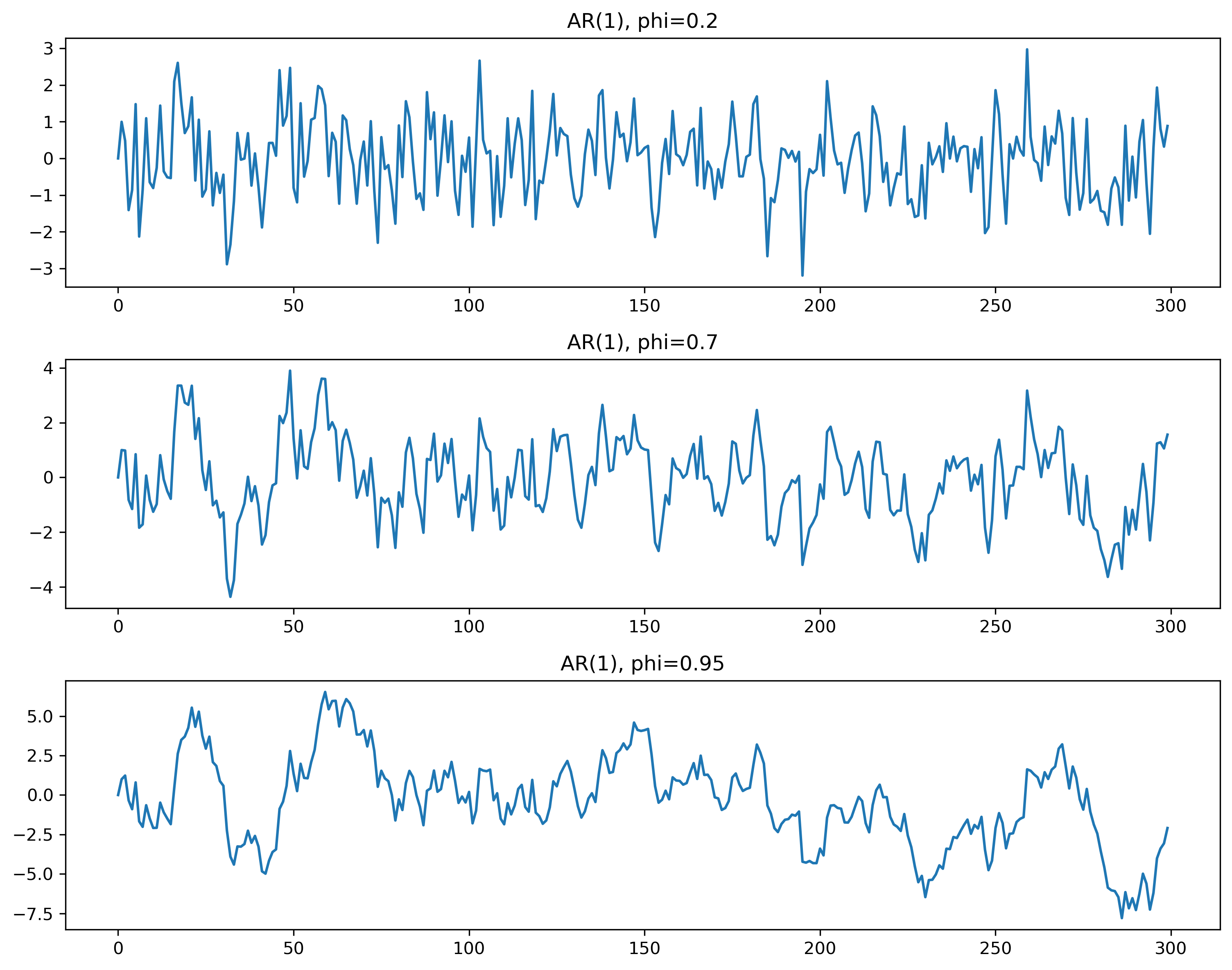

11.7 Variance¶

Var(x_t) = \frac{\sigma_w^2}{1-\phi^2}

11.8 ACF of AR(1)¶

\rho(h) = \phi^h

11.9 Simulated ACF¶

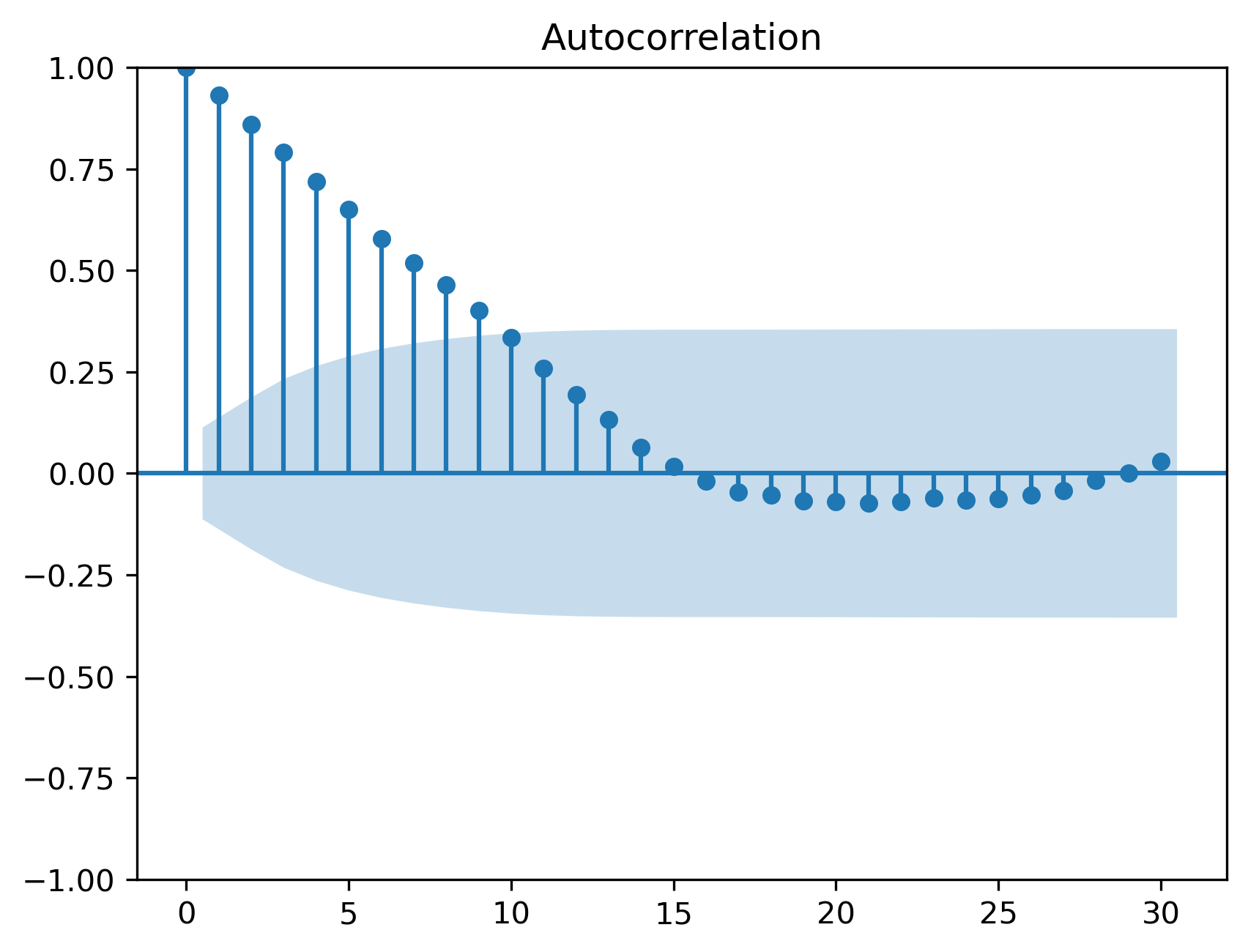
11.10 PACF of AR(1)¶

11.11 AR(2) Model¶

x_t = \phi_1 x_{t-1} + \phi_2 x_{t-2} + w_t

11.12 AR(2) Simulation¶

np.random.seed(123)

phi1, phi2 = 1.0, -0.6
n = 1000

w = np.random.normal(size=n)
x = np.zeros(n)

for t in range(2,n):
    x[t] = phi1*x[t-1] + phi2*x[t-2] + w[t]

plt.plot(x)
plt.title("AR(2)")

plt.savefig("figs/ch10/ar2.png", dpi=300, bbox_inches="tight")
plt.close()   # replace with plt.show()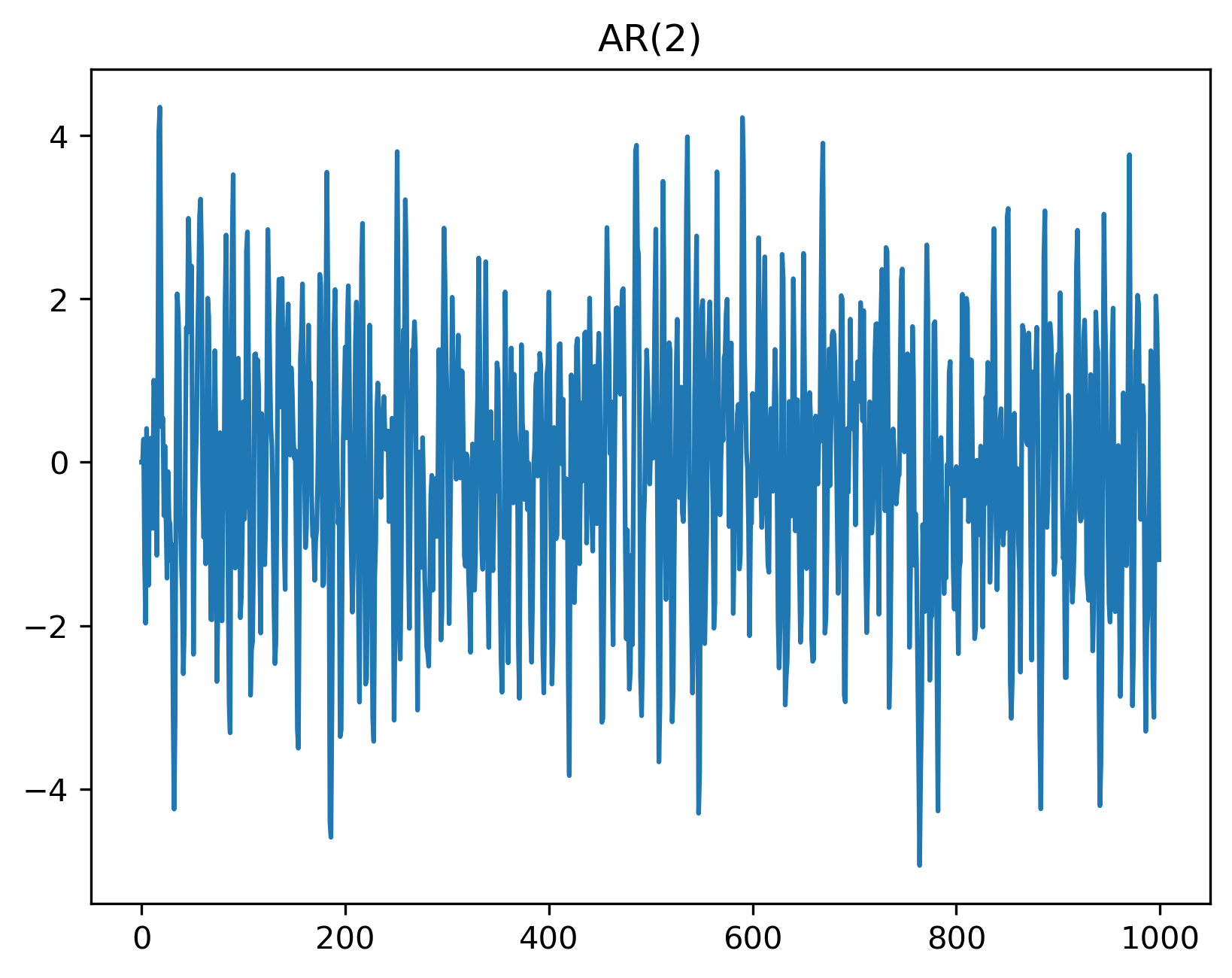

11.13 ACF and PACF for AR(2)¶

from statsmodels.graphics.tsaplots import plot_pacf

plot_acf(x, lags=30)
plot_pacf(x, lags=30)

plt.savefig("figs/ch11/ar2_acf_pacf.png", dpi=300, bbox_inches="tight")
plt.close()   # replace with plt.show()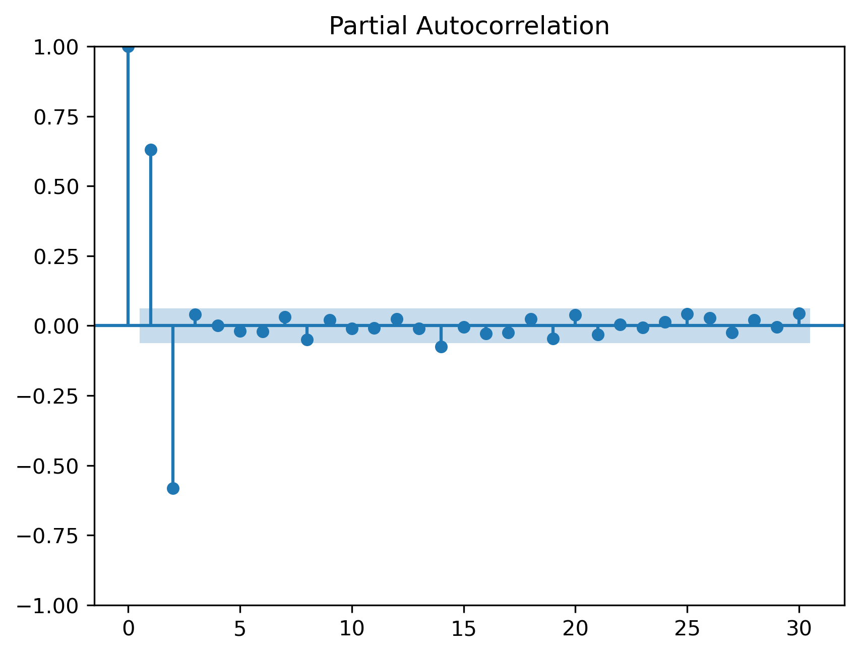

11.14 General AR(p)¶

x_t = \sum_{i=1}^p \phi_i x_{t-i} + w_t

11.15 Estimation in Python¶

                            AutoReg Model Results                             
==============================================================================
Dep. Variable:                      y   No. Observations:                 1000
Model:                     AutoReg(2)   Log Likelihood               -1416.520
Method:               Conditional MLE   S.D. of innovations              1.000
Date:                Mon, 04 May 2026   AIC                           2841.040
Time:                        21:40:24   BIC                           2860.663
Sample:                             2   HQIC                          2848.499
                                 1000                                         
==============================================================================
                 coef    std err          z      P>|z|      [0.025      0.975]
------------------------------------------------------------------------------
const         -0.0386      0.032     -1.218      0.223      -0.101       0.024
y.L1           1.0000      0.026     38.890      0.000       0.950       1.050
y.L2          -0.5850      0.026    -22.746      0.000      -0.635      -0.535
                                    Roots                                    
=============================================================================
                  Real          Imaginary           Modulus         Frequency
-----------------------------------------------------------------------------
AR.1            0.8547           -0.9894j            1.3074           -0.1366
AR.2            0.8547           +0.9894j            1.3074            0.1366
-----------------------------------------------------------------------------

11.16 Residual Diagnostics¶

|  | lb_stat   | lb_pvalue |
|---------|------------|-----------|
| 10      | 6.476702   | 0.773750  |
| 20      | 18.268325  | 0.569737  |

11.17 Information Criteria¶

AIC = -2\log L + 2k

BIC = -2\log L + k\log n

11.18 Common Mistakes¶

11.19 Looking Ahead¶

MA models
ARMA models
full modeling workflow

Key Takeaways¶

Concept Check¶

Basic¶

What is an autoregressive (AR) model?
What does the parameter $\phi$ represent in an AR(1) model?
What is the role of the error term $w_t$ ?

Intuition¶

What does it mean for a time series to exhibit persistence?
How does the value of $\phi$ affect the behavior of the series?
What happens when $\phi$ is:
- close to zero
- close to one
- negative

Intermediate¶

What is the stationarity condition for an AR(1) model?
Why must shocks decay over time in a stationary process?
What is the difference between:
- AR(1)
- AR(2)

ACF & PACF¶

What pattern does the ACF of an AR(1) process exhibit?
What pattern does the PACF of an AR(1) process exhibit?
Why does the PACF “cut off” for an AR process?

Finance Insight¶

Why are AR models useful in modeling economic or financial time series?
Why is strong persistence sometimes mistaken for a trend?

Challenge¶

Suppose $\phi = 0.98$ .

Is the process stationary?
How would it behave in practice?

Interpretation & Practice¶

A time series shows gradual adjustment after shocks.
- What type of model might describe this?
- Why?
A series appears highly persistent but does not trend upward.
- What does this suggest about $\phi$ ?
- Is the series likely stationary?
ACF decays slowly and smoothly.
- What type of process might this indicate?
PACF shows a large spike at lag 1 and near zero afterward.
- What model is suggested?
ACF shows a wavy, oscillating pattern.
- What type of model might generate this?
After fitting an AR model, residuals still show autocorrelation.
- What does this imply?
- What should you do?

Finance Interpretation¶

A return series shows small but positive autocorrelation.
- What does this imply about predictability?
- Is this consistent with market efficiency?
A volatility series shows strong persistence.
- Why might an AR-type structure be useful?

Challenge¶

A model fits the data well but produces poor forecasts.
- What might be wrong?
- What does this suggest about overfitting?

Numerical Practice¶

AR(1) Simulation Logic¶

Consider the AR(1) process:

x_t = 0.5 x_{t-1} + w_t

with:

$x_0 = 10$
$w_t = 2, -1, 3$

Compute $x_1, x_2, x_3$

Repeat with:

x_t = 0.9 x_{t-1} + w_t

Compare results
What changes?

Persistence¶

Suppose:

x_t = \phi x_{t-1} + w_t

If $\phi = 0.2$ , how quickly do shocks disappear?
If $\phi = 0.9$ , how quickly do shocks disappear?

ACF Interpretation¶

Suppose you observe:

$\rho(1) = 0.8$
$\rho(2) = 0.64$
$\rho(3) = 0.51$

What pattern is this?
What does it suggest about $\phi$ ?

Model Identification¶

You observe:

ACF gradually decays
PACF cuts off after lag 2

What model is suggested?

Estimation Output¶

Suppose an estimated AR(1) model gives:

x_t = 0.85 x_{t-1} + w_t

Is the series highly persistent?
Is it stationary?
What does this imply for forecasting?

Diagnostics¶

Suppose the residuals from an AR model show:

significant autocorrelation

What does this imply?
What should you do next?

Challenge¶

Suppose $\phi > 1$ .

What happens to the process?
Why is this problematic?

Suppose you include too many lags in an AR model.

What is the risk?
How can information criteria help?

Appendix 11A — Mathematical Details of AR Models¶

This appendix provides additional insight into the properties of autoregressive models.

These results are not required for basic understanding, but they help explain why AR models behave the way they do.

A.1 Recursive Representation of AR(1)¶

Consider:

x_t = \phi x_{t-1} + w_t

Substitute repeatedly:

x_t = \phi(\phi x_{t-2} + w_{t-1}) + w_t = \phi^2 x_{t-2} + \phi w_{t-1} + w_t

Continuing:

x_t = \sum_{j=0}^{\infty} \phi^j w_{t-j}

A.2 Stationarity Condition¶

From the recursive form:

x_t = \sum_{j=0}^{\infty} \phi^j w_{t-j}

For this to converge, we require:

|\phi| < 1

A.3 Mean of AR(1)¶

Consider:

x_t = \phi x_{t-1} + \mu + w_t

Take expectations:

E[x_t] = \phi E[x_{t-1}] + \mu

In equilibrium:

E[x_t] = E[x_{t-1}] = \bar{x}

So:

\bar{x} = \phi \bar{x} + \mu

\bar{x} = \frac{\mu}{1-\phi}

A.4 Variance of AR(1)¶

From:

x_t = \phi x_{t-1} + w_t

Take variance:

Var(x_t) = \phi^2 Var(x_{t-1}) + \sigma_w^2

In steady state:

Var(x_t) = \sigma_x^2

So:

\sigma_x^2 = \phi^2 \sigma_x^2 + \sigma_w^2

\sigma_x^2 = \frac{\sigma_w^2}{1-\phi^2}

A.5 Autocovariance Function¶

We define:

\gamma(h) = Cov(x_t, x_{t-h})

Multiply the AR(1) equation by $x_{t-h}$ :

Cov(x_t, x_{t-h}) = \phi Cov(x_{t-1}, x_{t-h})

Thus:

\gamma(h) = \phi \gamma(h-1)

Iterating:

\gamma(h) = \phi^h \gamma(0)

A.6 Autocorrelation Function¶

Since:

\rho(h) = \frac{\gamma(h)}{\gamma(0)}

we obtain:

\rho(h) = \phi^h

A.7 Yule–Walker Equation (AR(1))¶

At lag 0:

\gamma(0) = \phi^2 \gamma(0) + \sigma_w^2

Rearranging:

\gamma(0) (1 - \phi^2) = \sigma_w^2

This gives the variance result above.

A.8 AR(2): Intuition and Dynamics¶

Consider:

x_t = \phi_1 x_{t-1} + \phi_2 x_{t-2} + w_t

Unlike AR(1), this process can generate:

oscillations
cycles
damped fluctuations

A.9 Characteristic Equation¶

For AR(p):

x_t = \phi_1 x_{t-1} + \cdots + \phi_p x_{t-p} + w_t

We define the characteristic equation:

1 - \phi_1 z - \phi_2 z^2 - \cdots - \phi_p z^p = 0

Chapter 11 — Autoregressive Models

Learning Objectives¶

11.1 The Basic Idea¶

11.2 The AR(1) Model¶

Mean¶

11.3 Mean-Centered Form¶

11.4 Recursive Representation (Key Insight)¶

11.5 Stationarity¶

11.6 Simulation¶

11.7 Variance¶

11.8 ACF of AR(1)¶

11.9 Simulated ACF¶

11.10 PACF of AR(1)¶

11.11 AR(2) Model¶

11.12 AR(2) Simulation¶

11.13 ACF and PACF for AR(2)¶

11.14 General AR(p)¶

11.15 Estimation in Python¶

11.16 Residual Diagnostics¶

11.17 Information Criteria¶

11.18 Common Mistakes¶

11.19 Looking Ahead¶

Key Takeaways¶

Concept Check¶

Basic¶

Intuition¶

Intermediate¶

ACF & PACF¶

Finance Insight¶

Challenge¶

Interpretation & Practice¶

Finance Interpretation¶

Challenge¶

Numerical Practice¶

AR(1) Simulation Logic¶

Persistence¶

ACF Interpretation¶

Model Identification¶

Estimation Output¶

Diagnostics¶

Challenge¶

Appendix 11A — Mathematical Details of AR Models¶

A.1 Recursive Representation of AR(1)¶

A.2 Stationarity Condition¶

A.3 Mean of AR(1)¶

A.4 Variance of AR(1)¶

A.5 Autocovariance Function¶

A.6 Autocorrelation Function¶

A.7 Yule–Walker Equation (AR(1))¶

A.8 AR(2): Intuition and Dynamics¶

A.9 Characteristic Equation¶

A.10 Why This Matters¶