Chapter 3 — A Quick Review of Probability and Statistics

Time series analysis combines:

data,
uncertainty,
randomness,
and statistical inference.

Before studying dynamic models, we briefly review several statistical ideas that will appear repeatedly throughout the book.

This chapter is intentionally intuitive and applications-oriented.

The goal is not to provide a complete statistics course.

Instead, the goal is to build enough intuition to understand uncertainty in time series analysis.

We will focus on ideas that are especially important in economics, finance, and forecasting.

Learning Objectives¶

By the end of this chapter, you should be able to:

explain the meaning of randomness
distinguish populations from samples
understand probability distributions intuitively
interpret the mean and variance
understand the normal distribution
understand why fat tails matter in finance
interpret hypothesis tests and p-values intuitively
understand statistical uncertainty in estimation and forecasting

3.1 Why Probability Matters¶

Economic and financial systems are uncertain.

Examples include:

tomorrow’s stock return,
next month’s inflation,
future GDP growth,
exchange rate movements,
financial crises.

We therefore cannot predict outcomes with certainty.

Instead, we reason probabilistically.

3.2 Random Variables¶

A random variable is a variable whose future value is uncertain.

Examples include:

tomorrow’s stock return,
next quarter’s GDP growth,
next month’s inflation rate.

We often denote a random variable by:

X

Possible outcomes may include:

x_1,x_2,x_3,\dots

Example: Stock Returns¶

Suppose tomorrow’s stock return could be:

Outcome	Probability
+2%	0.4
0%	0.3
-3%	0.3

The future return is uncertain.

Probability describes how likely different outcomes are.

3.3 Populations and Samples¶

In statistics, we often distinguish between:

populations,
and samples.

Population¶

A population represents the entire set of possible observations.

Example:

all daily returns that could ever occur.

Sample¶

A sample is the observed subset of data.

Example:

daily stock returns from 2020–2024.

3.4 Mean and Expected Value¶

The mean measures the center of a distribution.

For observations:

x_1,x_2,\dots,x_n

the sample mean is:

\bar{x} = \frac{1}{n} \sum_{i=1}^{n}x_i

Interpretation¶

The mean measures the average level of the data.

Examples:

average inflation,
average GDP growth,
average stock return.

Expected Value¶

For random variables, the theoretical average is called the expected value.

E[X]

3.5 Variance and Volatility¶

The mean alone is not enough.

Two variables may have the same average but very different uncertainty.

Variance measures dispersion around the mean.

Variance¶

The sample variance is:

s^2 = \frac{1}{n-1} \sum_{i=1}^{n}(x_i-\bar{x})^2

The standard deviation is:

s=\sqrt{s^2}

Financial Interpretation¶

In finance, volatility is often measured using the standard deviation of returns.

Higher volatility means:

larger fluctuations,
greater uncertainty,
greater risk.

3.6 Probability Distributions¶

A probability distribution describes how likely different outcomes are.

Different variables may follow different distributions.

Examples¶

Variable	Typical Distribution Shape
heights	roughly normal
income	right-skewed
stock returns	fat-tailed
waiting times	asymmetric

3.7 The Normal Distribution¶

The normal distribution is one of the most important probability distributions in statistics.

It is symmetric and bell-shaped.

X \sim N(\mu,\sigma^2)

means:

mean = $\mu$
variance = $\sigma^2$

Properties of the Normal Distribution¶

The normal distribution is:

symmetric,
smooth,
fully characterized by mean and variance.

The 68–95–99.7 Rule¶

For a normal distribution:

Range	Approximate Probability
within 1 standard deviation	68%
within 2 standard deviations	95%
within 3 standard deviations	99.7%

3.8 Why Finance Often Violates Normality¶

Financial returns often display:

extreme movements,
crashes,
sudden rallies,
volatility clustering.

Large events occur more often than predicted by the normal distribution.

This phenomenon is called:

fat tails

Example¶

Stock market crashes are much more common than a simple normal model would predict.

This observation motivates later volatility models such as ARCH and GARCH.

3.9 The t Distribution¶

The t distribution resembles the normal distribution but has fatter tails.

It is especially useful when:

sample sizes are small,
uncertainty about variance is important.

Intuition¶

Compared with the normal distribution:

moderate observations behave similarly,
extreme observations become more likely.

3.10 The F Distribution¶

The F distribution commonly appears when comparing:

variances,
regression models,
joint restrictions.

For now, the important point is conceptual:

We will encounter F-tests later in regression and VAR models.

3.11 Sampling Uncertainty¶

Suppose we estimate average stock returns using historical data.

If we choose a different sample period, the estimated mean may differ.

This is called sampling uncertainty.

Example¶

Average returns estimated from:

2010–2015,
2015–2020,
2020–2025

may differ substantially.

3.12 Statistical Inference¶

Statistical inference uses sample data to make statements about broader populations.

Examples include:

Is average inflation increasing?
Is stock market volatility unusually high?
Does a forecasting model outperform another model?

Inference therefore combines:

estimation,
uncertainty,
probability.

3.13 Hypothesis Testing¶

A hypothesis test evaluates whether the data support a particular claim.

Example¶

Suppose we test:

H_0:\mu=0

against:

H_1:\mu \neq 0

where:

$H_0$ = null hypothesis
$H_1$ = alternative hypothesis

Financial Interpretation¶

For example:

H_0:\text{average return}=0

asks whether average returns differ significantly from zero.

3.14 Test Statistic¶

A test statistic summarizes how far the data deviate from the null hypothesis.

For example, a t-statistic often takes the form:

t = \frac{ \text{observed} - \text{expected value} }{ \text{standard error} }

Large values suggest stronger evidence against the null hypothesis.

3.15 p-Values¶

A p-value measures how surprising the observed data would be if the null hypothesis were true.

Small p-values imply stronger evidence against the null hypothesis.

Common Rule¶

p-value	Interpretation
small	evidence against $H_0$
large	insufficient evidence against $H_0$

This is a very common misunderstanding.

3.16 Confidence Intervals¶

A confidence interval provides a plausible range for an unknown parameter.

For example:

Average inflation is estimated to be 2.5% ± 0.5%.

This communicates uncertainty more clearly than a single number.

3.17 Correlation¶

Correlation measures how strongly two variables move together.

The correlation coefficient is often denoted:

\rho

or:

r

Interpretation¶

Correlation	Meaning
+1	perfect positive relationship
0	no linear relationship
-1	perfect negative relationship

Financial Examples¶

Correlations matter greatly in finance because diversification depends on how assets move together.

Two variables may move together without one causing the other.

3.18 Randomness vs Predictability¶

A central challenge in time series analysis is distinguishing:

genuine structure,
from random noise.

Some movements may be predictable.

Others may simply reflect randomness.

This question appears repeatedly throughout time series analysis.

3.19 Simulating Random Data in Python¶

We now simulate random observations from a normal distribution.

import numpy as np
import matplotlib.pyplot as plt

np.random.seed(123)

x = np.random.normal(size=1000)

plt.hist(x, bins=30)

plt.title("Simulated Normal Data")

plt.savefig("figs/ch3/normal.png", dpi=300, bbox_inches="tight")
plt.close()   # replace with plt.show()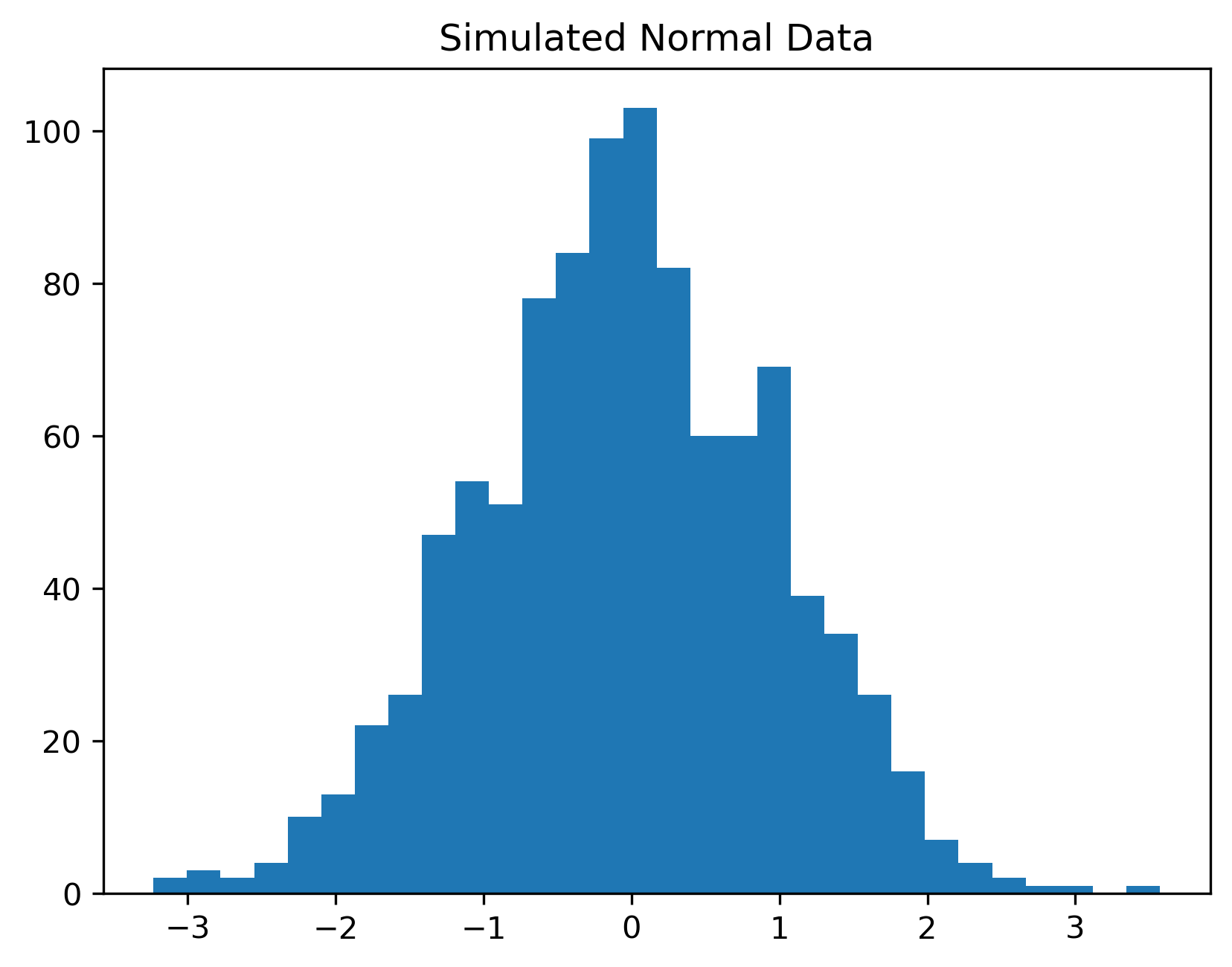

This is an important lesson in time series analysis.

3.20 Simulating Fat Tails¶

We now compare the normal distribution with a t distribution.

import numpy as np
import matplotlib.pyplot as plt

np.random.seed(123)

normal = np.random.normal(size=10000)

t_dist = np.random.standard_t(df=3, size=10000)

plt.hist(normal, bins=60, alpha=0.5, density=True, label="Normal")

plt.hist(t_dist, bins=60, alpha=0.5, density=True, label="t(3)")

plt.legend()

plt.title("Normal vs Fat-Tailed t Distribution")

plt.savefig("figs/ch3/fattail.png", dpi=300, bbox_inches="tight")
plt.close()   # replace with plt.show()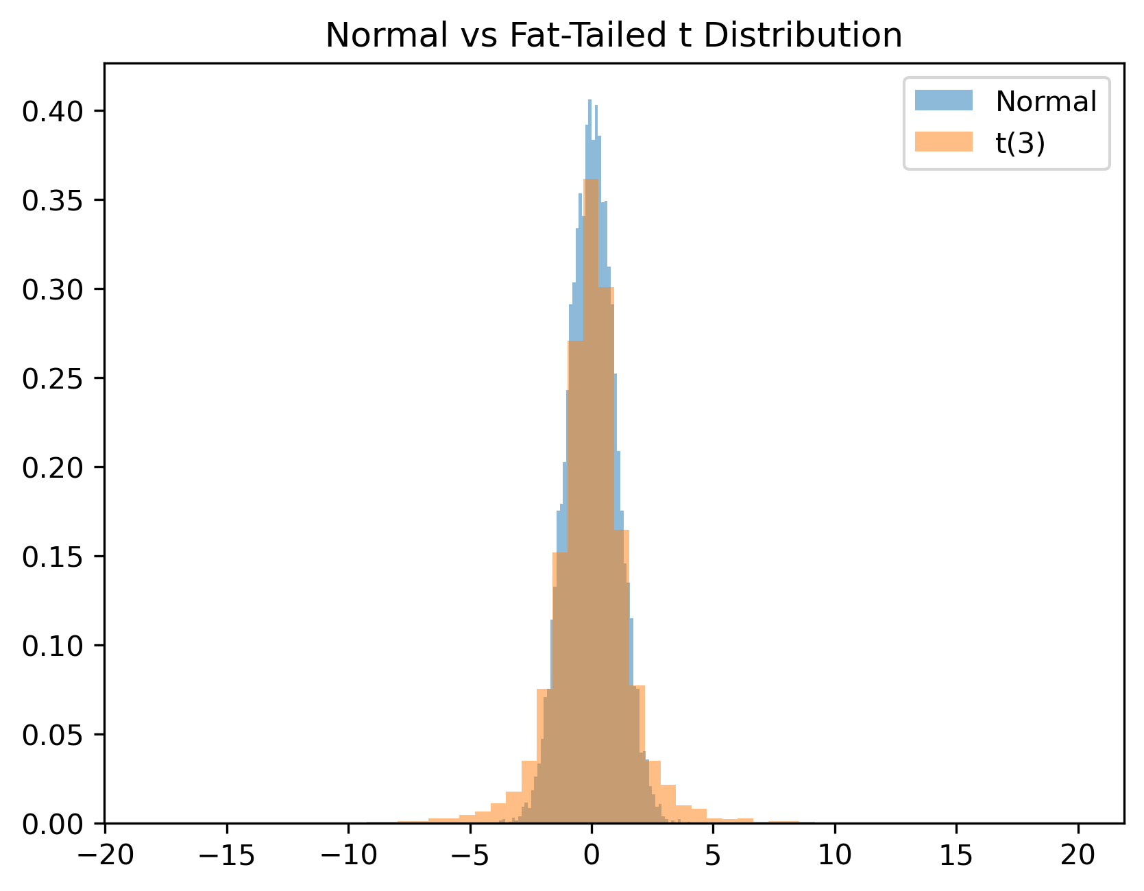

This helps explain why financial returns often appear more volatile than standard textbook models predict.

3.21 Gretl Example: Descriptive Statistics¶

Gretl can quickly compute descriptive statistics.

Step 1: Open Data¶

Load a dataset.

Step 2: Summary Statistics¶

Menu:

View → Summary statistics

GRETL reports:

mean
standard deviation
minimum
maximum
skewness
kurtosis

[GRETL Screenshot Placeholder: Summary statistics window]

3.22 Common Mistakes¶

3.23 Looking Ahead¶

This chapter reviewed several statistical ideas that will appear repeatedly throughout the book.

We now begin studying how to visualize and interpret time series data directly.

The next chapter introduces:

plotting time series,
trends,
cycles,
rolling averages,
and visual pattern detection.

Key Takeaways¶

Concept Check¶

Basic¶

What is a probability distribution?
What does the mean of a distribution represent?
What does the standard deviation measure?

Intuition¶

Why is randomness unavoidable in economic and financial data?
What does it mean for an event to be “unlikely”?
Why do financial returns often exhibit more extreme outcomes than the normal distribution predicts?

Intermediate¶

What is the 68–95–99.7 rule?
Why is the normal distribution often used as a benchmark in finance?
What is a p-value?
Why does a small p-value provide evidence against a null hypothesis?

Challenge¶

A model assumes returns are normally distributed.

Why might this assumption underestimate risk?
What type of events become more likely in reality?

Interpretation & Practice¶

A histogram of returns appears roughly bell-shaped but shows a few very large spikes.
- What does this suggest about the distribution?
- Why might the normal model be misleading here?

Suppose returns are centered around zero but fluctuate widely.
- What does this imply about risk?
- Why might investors still be concerned?

A risk model predicts that extreme losses are “very unlikely.”
- What assumption is likely being made?
- Why might this be dangerous in practice?

A hypothesis test produces:
p-value = 0.04
- What is the decision at the 5% level?
- What does this imply about the null hypothesis?

A hypothesis test produces:
p-value = 0.25
- What does this imply?
- Why does this NOT prove the null hypothesis is true?

Challenge¶

Suppose a financial model consistently underpredicts large losses.
- What feature of the data is the model likely missing?
- Why is this especially problematic in finance?

Numerical Practice¶

Basic¶

Suppose a variable has:
mean = 100
standard deviation = 15
- Using the 68–95–99.7 rule, what range contains about 95% of observations?

Using the same distribution:
- Is a value of 130 likely or unlikely?
- Roughly what percentage of observations exceed 130?

Intermediate¶

Suppose returns follow a normal distribution with:
mean = 0
standard deviation = 2
- What range contains about 68% of returns?
- What range contains about 95% of returns?

Two assets have:
Asset Mean Return Standard Deviation
A 2% 5%
B 3% 5%
- Which asset would a risk-neutral investor prefer?
- Why?

Asset	Mean Return	Standard Deviation
A	2%	5%
B	3%	5%

Two assets have:
Asset Mean Return Standard Deviation
C 3% 4%
D 3% 8%
- Which asset is riskier?
- Why might an investor prefer Asset C?

Asset	Mean Return	Standard Deviation
C	3%	4%
D	3%	8%

Hypothesis Testing¶

6. Testing Average Return¶

A trader claims that a strategy generates a positive average daily return.

You collect a sample of 25 daily returns with:

sample mean = 0.8%
sample standard deviation = 2%

State the null and alternative hypotheses.
Compute the test statistic:

t = \frac{\bar{r} - 0}{s / \sqrt{n}}

Using a 5% significance level (critical value ≈ 2), do you reject the null?
What is your economic conclusion?

7. Testing for Zero Mean¶

An analyst believes that a stock’s average return is zero.

You observe:

sample mean = 0.3%
sample standard deviation = 1.5%
sample size = 100

State the null and alternative hypotheses.
Compute the test statistic.
Is the result statistically significant at the 5% level?
Does statistical significance imply the strategy is economically meaningful?

8. Volatility Change (Interpretation Focus)¶

Suppose two periods of returns have:

Period	Mean Return	Standard Deviation
A	0.5%	1%
B	0.5%	3%

Would you expect more extreme outcomes in Period A or B?
If a model assumes constant variance, what mistake might it make?

Challenge¶

A risk model assumes returns are normally distributed with:

mean = 0
standard deviation = 2
Using the 68–95–99.7 rule, what is the approximate probability of a return less than −6?
If actual data show more such extreme events, what does this imply about the model?
Why is this important for financial risk management?