Part VIII Capstone — Forecasting Volatility and Financial Risk
In Part VIII, we studied models for time-varying volatility:
ARCH models,
GARCH models,
volatility clustering,
conditional variance,
and volatility forecasting.
This capstone applies these ideas to daily financial returns.
We use SPY, an ETF tracking the S&P 500.
Exercise 1 — Download Price Data
import yfinance as yf
import numpy as np
import pandas as pd
import matplotlib.pyplot as plt

spy = yf.download(
    "SPY",
    start="2015-01-01",
    auto_adjust=False
)

prices = spy["Adj Close"].squeeze()

prices.plot(figsize=(10,4))

plt.title("SPY Adjusted Closing Prices")
plt.ylabel("Price")
plt.xlabel("Date")

plt.savefig("figs/ch26_/SPY.png", dpi=300, bbox_inches="tight")
plt.close()   # replace with plt.show()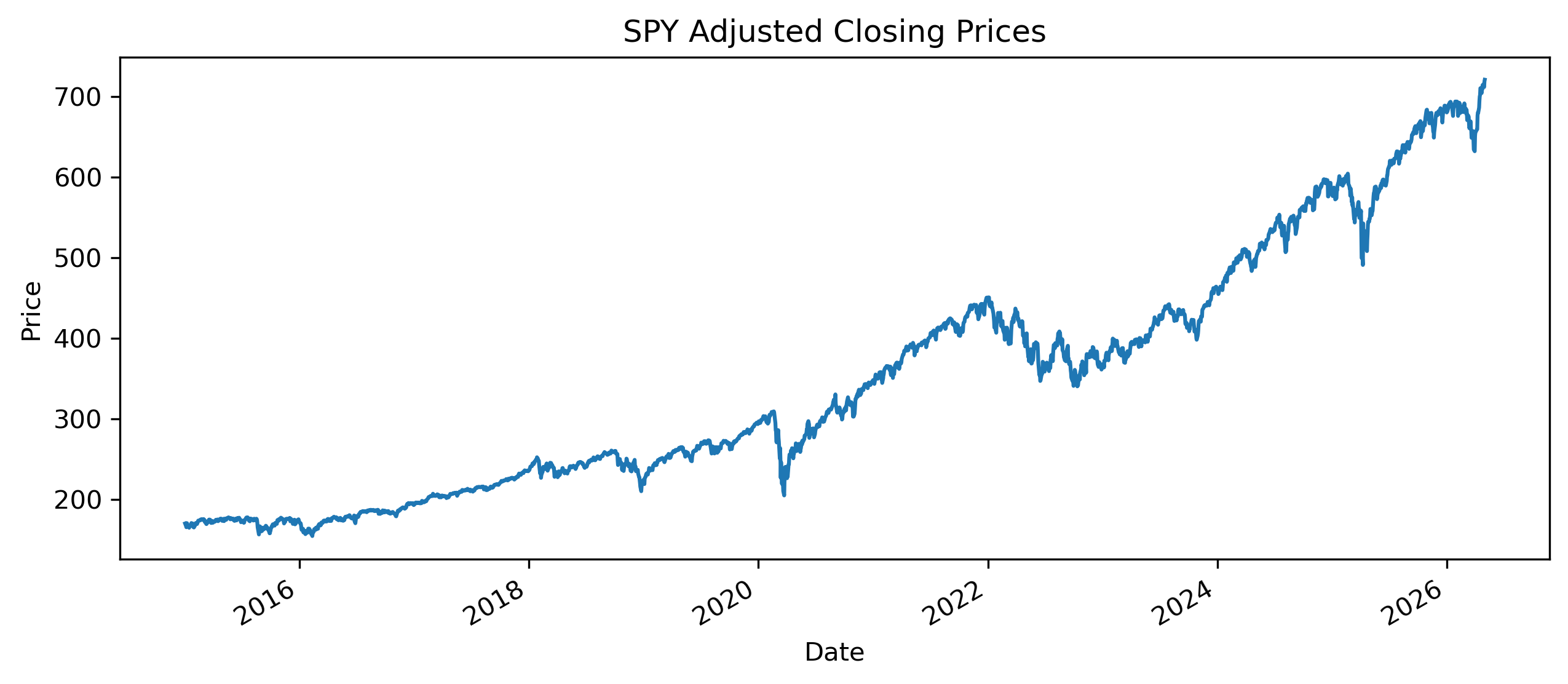
Exercise 2 — Compute Log Returns
returns = 100 * np.log(
    prices / prices.shift(1)
)

returns = returns.dropna()

returns.plot(figsize=(10,4))

plt.title("SPY Daily Log Returns")
plt.ylabel("Return (%)")
plt.xlabel("Date")

plt.savefig("figs/ch26_/rtn.png", dpi=300, bbox_inches="tight")
plt.close()   # replace with plt.show()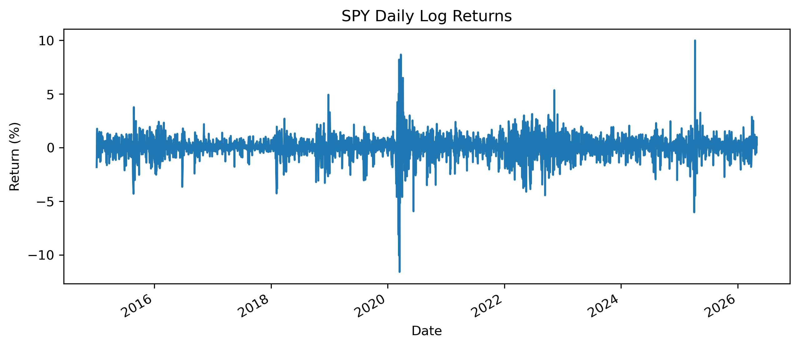
Exercise 3 — Rolling Volatility
rolling_vol = returns.rolling(30).std()

rolling_vol.plot(figsize=(10,4))

plt.title("30-Day Rolling Volatility")
plt.ylabel("Volatility")
plt.xlabel("Date")

plt.savefig("figs/ch26_/rol_vol.png", dpi=300, bbox_inches="tight")
plt.close()   # replace with plt.show()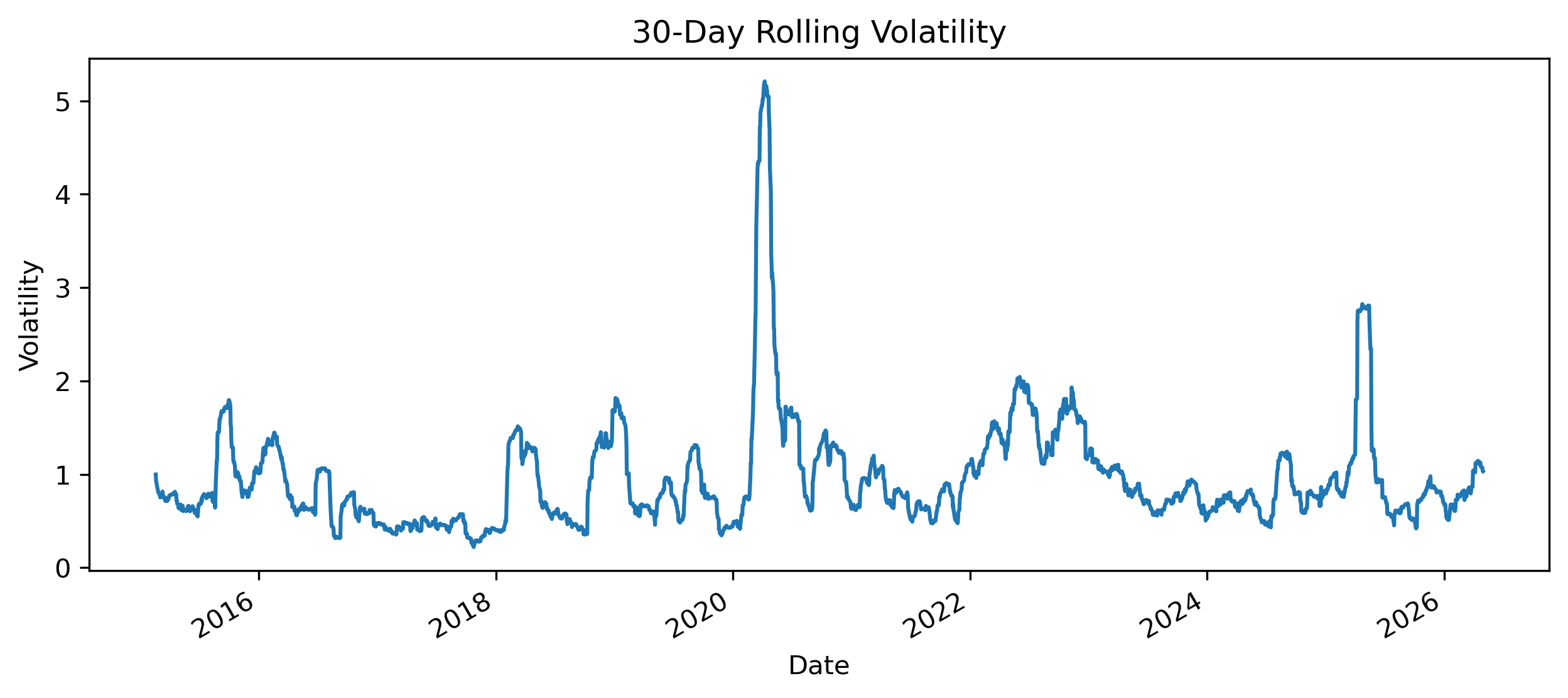
Exercise 4 — Testing for ARCH Effects
from statsmodels.stats.diagnostic import het_arch

arch_test = het_arch(
    returns,
    nlags=10
)

print("LM Statistic:", arch_test[0])
print("LM Test p-value:", arch_test[1])
print("F Statistic:", arch_test[2])
print("F Test p-value:", arch_test[3])
LM Statistic: 848.0078628375993
LM Test p-value: 9.790554714049502e-176
F Statistic: 120.46872866846164
F Test p-value: 1.6667139182935798e-209Exercise 5 — Install and Load the ARCH Package
Exercise 6 — Estimate a GARCH(1,1) Model
from arch import arch_model

garch_model = arch_model(
    returns,
    mean="Constant",
    vol="GARCH",
    p=1,
    q=1,
    dist="normal"
)

garch_results = garch_model.fit(
    disp="off"
)

print(garch_results.summary())
Constant Mean - GARCH Model Results
==============================================================================
Dep. Variable: SPY R-squared: 0.000
Mean Model: Constant Mean Adj. R-squared: 0.000
Vol Model: GARCH Log-Likelihood: -3671.36
Distribution: Normal AIC: 7350.72
Method: Maximum Likelihood BIC: 7374.53
No. Observations: 2848
Date: Sun, May 03 2026 Df Residuals: 2847
Time: 23:25:08 Df Model: 1
Mean Model
==========================================================================
coef std err t P>|t| 95.0% Conf. Int.
--------------------------------------------------------------------------
mu 0.0851 1.401e-02 6.079 1.208e-09 [5.769e-02, 0.113]
Volatility Model
============================================================================
coef std err t P>|t| 95.0% Conf. Int.
----------------------------------------------------------------------------
omega 0.0405 1.034e-02 3.918 8.926e-05 [2.026e-02,6.081e-02]
alpha[1] 0.1764 2.711e-02 6.508 7.629e-11 [ 0.123, 0.230]
beta[1] 0.7907 2.803e-02 28.213 4.059e-175 [ 0.736, 0.846]
============================================================================
Covariance estimator: robustExercise 7 — Plot Conditional Volatility
conditional_vol = garch_results.conditional_volatility

conditional_vol.plot(figsize=(10,4))

plt.title("Estimated GARCH Conditional Volatility")
plt.ylabel("Volatility")
plt.xlabel("Date")

plt.savefig("figs/ch26_/garch11.png", dpi=300, bbox_inches="tight")
plt.close()   # replace with plt.show()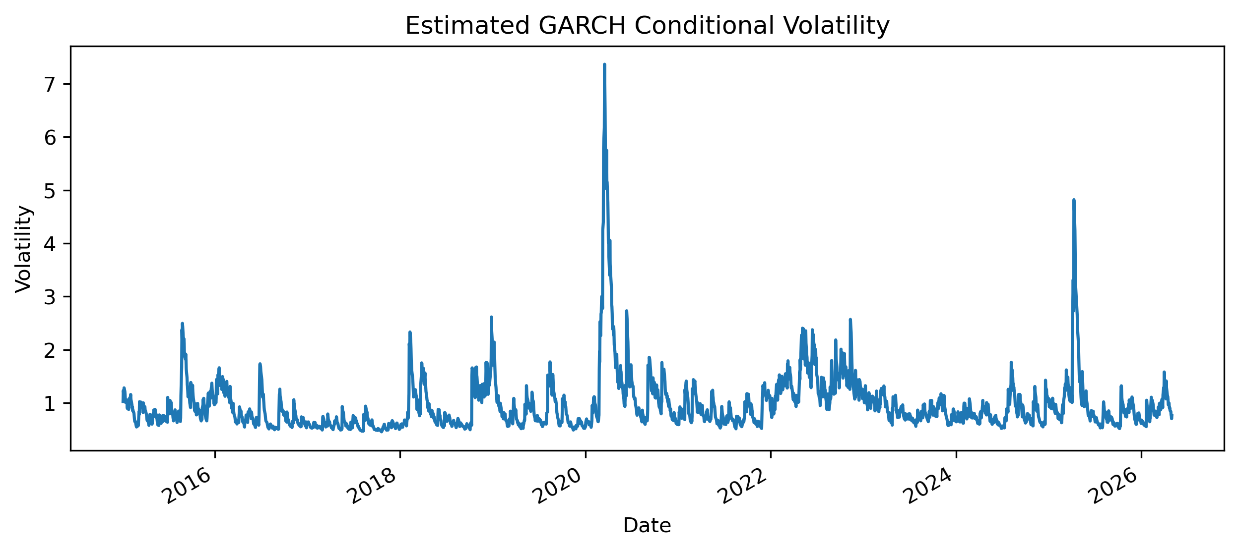
Exercise 8 — Compare Returns and Conditional Volatility
fig, ax1 = plt.subplots(figsize=(10,5))

ax1.plot(
    returns,
    label="Returns",
    alpha=0.6
)

ax1.set_ylabel("Return (%)")

ax2 = ax1.twinx()

ax2.plot(
    conditional_vol,
    label="Conditional Volatility",
    linestyle="--"
)

ax2.set_ylabel("Volatility")

plt.title("Returns and GARCH Conditional Volatility")

plt.savefig("figs/ch26_/garch11_r.png", dpi=300, bbox_inches="tight")
plt.close()   # replace with plt.show()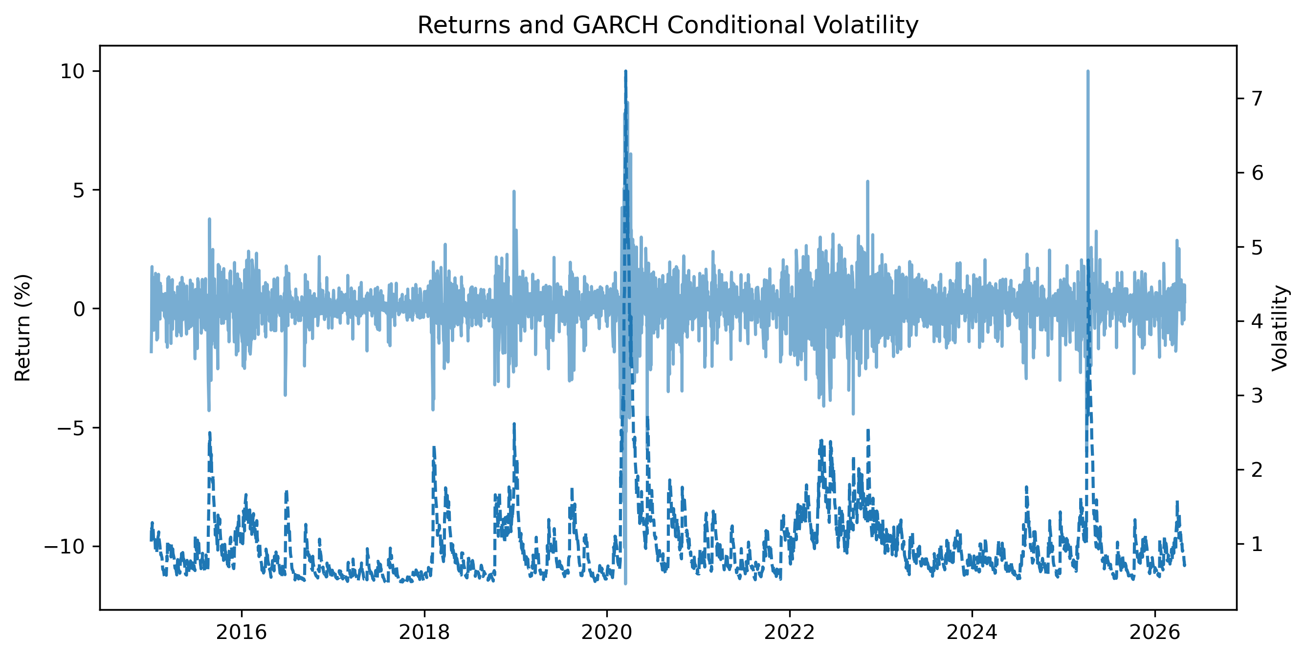
Exercise 9 — Forecast Volatility
forecast = garch_results.forecast(
    horizon=10
)

variance_forecast = forecast.variance.iloc[-1]

vol_forecast = np.sqrt(variance_forecast)

vol_forecast
h.01 0.708746
h.02 0.725500
h.03 0.741344
h.04 0.756351
h.05 0.770588
h.06 0.784110
h.07 0.796971
h.08 0.809214
h.09 0.820882
h.10 0.832011Exercise 10 — Plotting Recent Volatility and the Forecast
We now compare:
recent estimated volatility,
and the 10-day ahead volatility forecast.
This helps visualize how GARCH models project volatility into the future.
# ==========================================
# Extract recent volatility history
# ==========================================

recent_vol = conditional_vol.iloc[-100:]

# ==========================================
# Forecast future volatility
# ==========================================

forecast = garch_results.forecast(
    horizon=10
)

forecast_var = forecast.variance.iloc[-1]

forecast_vol = np.sqrt(forecast_var)

# ==========================================
# Construct forecast index
# ==========================================

forecast_index = range(
    len(recent_vol),
    len(recent_vol) + len(forecast_vol)
)

# ==========================================
# Plot
# ==========================================

plt.figure(figsize=(10,5))

# Historical volatility
plt.plot(
    range(len(recent_vol)),
    recent_vol,
    label="Historical Volatility",
    linewidth=2
)

# Forecast volatility
plt.plot(
    forecast_index,
    forecast_vol,
    label="Forecast Volatility",
    linewidth=2,
    linestyle="--"
)

plt.title("Recent and Forecast GARCH Volatility")

plt.ylabel("Volatility")

plt.xlabel("Time")

plt.legend()

plt.show()Exercise 11 — Simple Value-at-Risk
We compute a simple one-day 5% Value-at-Risk.
latest_vol = conditional_vol.iloc[-1]

var_5 = -1.645 * latest_vol

print("One-day 5% VaR:", var_5)
One-day 5% VaR: -1.2482842037087853Exercise 12 — Common Mistakes
Key Takeaways